11 755 Machine Learning for Signal Processing Expectation

11 -755 Machine Learning for Signal Processing Expectation Maximization Mixture Models HMMs Class 9. 21 Sep 2010 11755/18797 1

Learning Distributions for Data n Problem: Given a collection of examples from some data, estimate its distribution q Basic ideas of Maximum Likelihood and MAP estimation can be found in Aarti/Paris’ slides n n Solution: Assign a model to the distribution q n n Learn parameters of model from data Models can be arbitrarily complex q n Pointed to in a previous class Mixture densities, Hierarchical models. Learning must be done using Expectation Maximization Following slides: An intuitive explanation using a simple example of multinomials 21 Sep 2010 11755/18797 2

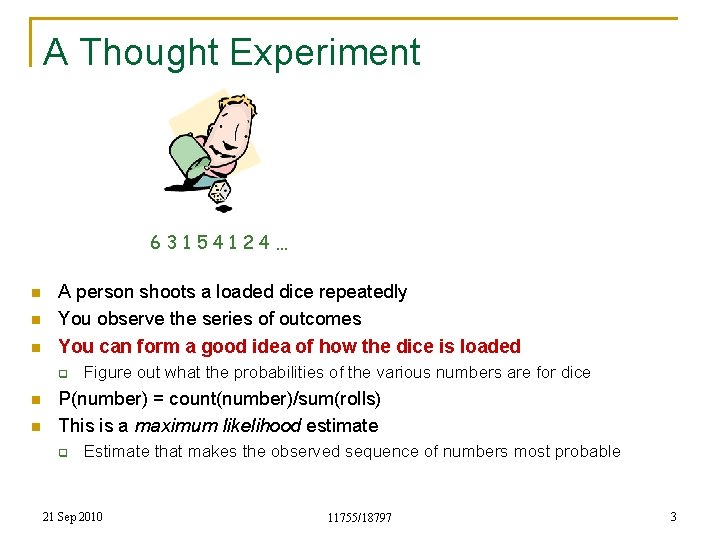
A Thought Experiment 63154124… n n n A person shoots a loaded dice repeatedly You observe the series of outcomes You can form a good idea of how the dice is loaded q n n Figure out what the probabilities of the various numbers are for dice P(number) = count(number)/sum(rolls) This is a maximum likelihood estimate q Estimate that makes the observed sequence of numbers most probable 21 Sep 2010 11755/18797 3

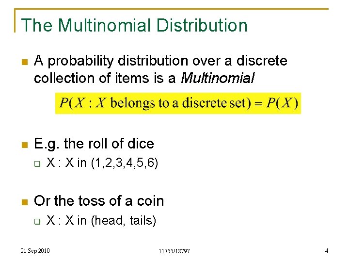
The Multinomial Distribution n A probability distribution over a discrete collection of items is a Multinomial n E. g. the roll of dice q n X : X in (1, 2, 3, 4, 5, 6) Or the toss of a coin q X : X in (head, tails) 21 Sep 2010 11755/18797 4

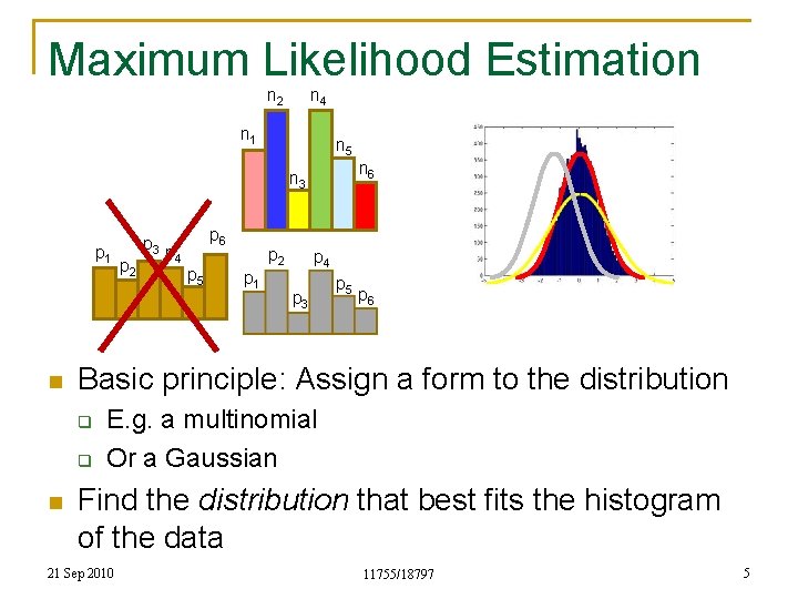
Maximum Likelihood Estimation n 2 n 4 n 1 n 5 n 6 n 3 p 1 n p 4 p 6 p 5 p 2 p 1 p 4 p 3 p 5 p 6 Basic principle: Assign a form to the distribution q q n p 2 p 3 E. g. a multinomial Or a Gaussian Find the distribution that best fits the histogram of the data 21 Sep 2010 11755/18797 5

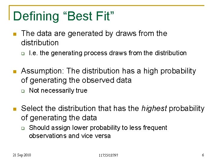
Defining “Best Fit” n The data are generated by draws from the distribution q n Assumption: The distribution has a high probability of generating the observed data q n I. e. the generating process draws from the distribution Not necessarily true Select the distribution that has the highest probability of generating the data q Should assign lower probability to less frequent observations and vice versa 21 Sep 2010 11755/18797 6

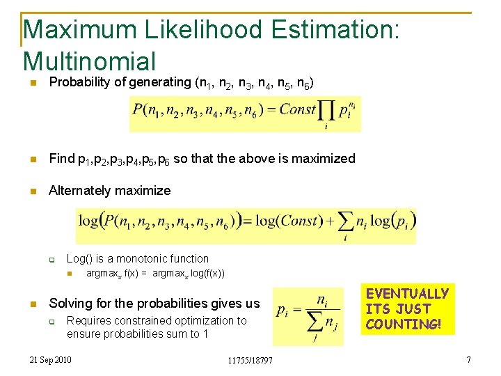
Maximum Likelihood Estimation: Multinomial n Probability of generating (n 1, n 2, n 3, n 4, n 5, n 6) n Find p 1, p 2, p 3, p 4, p 5, p 6 so that the above is maximized n Alternately maximize q Log() is a monotonic function n n argmaxx f(x) = argmaxx log(f(x)) Solving for the probabilities gives us q Requires constrained optimization to ensure probabilities sum to 1 21 Sep 2010 11755/18797 EVENTUALLY ITS JUST COUNTING! 7

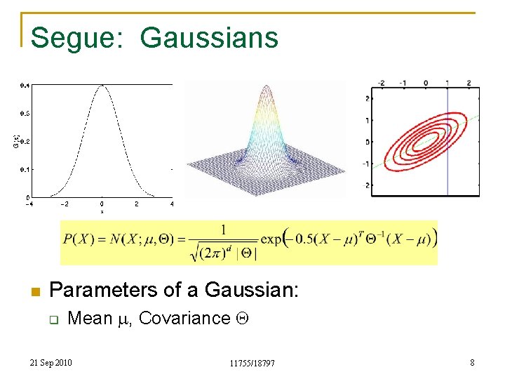
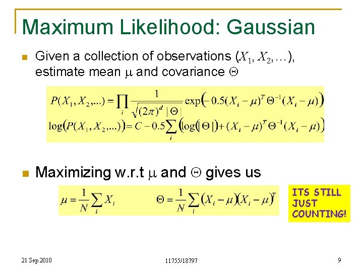
Segue: Gaussians n Parameters of a Gaussian: q Mean m, Covariance Q 21 Sep 2010 11755/18797 8

Maximum Likelihood: Gaussian n n Given a collection of observations (X 1, X 2, …), estimate mean m and covariance Q Maximizing w. r. t m and Q gives us ITS STILL JUST COUNTING! 21 Sep 2010 11755/18797 9

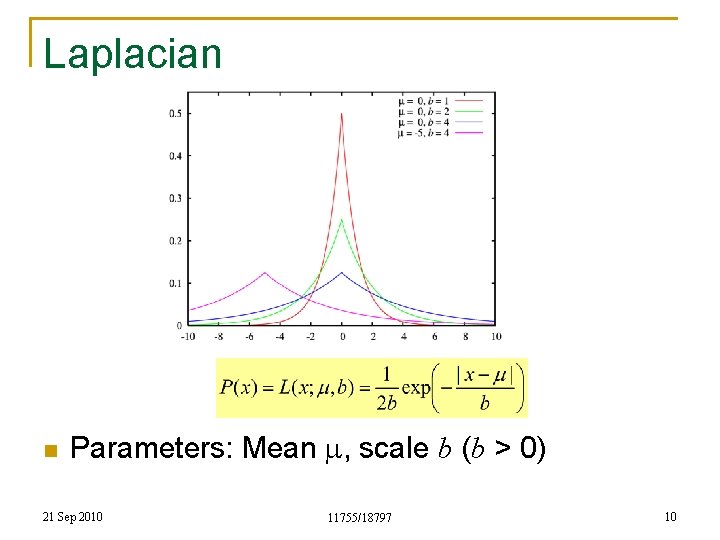
Laplacian n Parameters: Mean m, scale b (b > 0) 21 Sep 2010 11755/18797 10

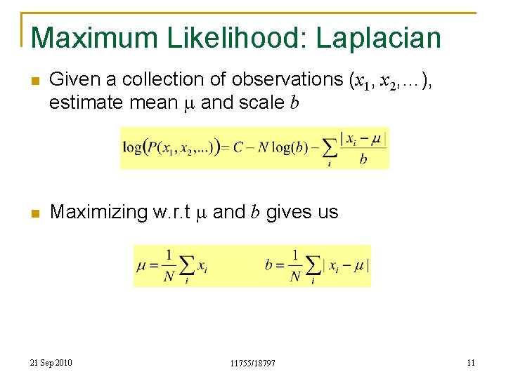
Maximum Likelihood: Laplacian n n Given a collection of observations (x 1, x 2, …), estimate mean m and scale b Maximizing w. r. t m and b gives us 21 Sep 2010 11755/18797 11

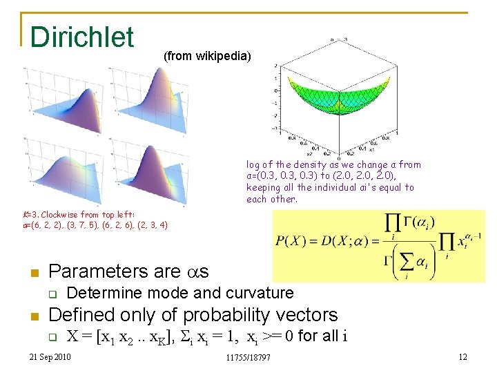
Dirichlet (from wikipedia) log of the density as we change α from α=(0. 3, 0. 3) to (2. 0, 2. 0), keeping all the individual αi's equal to each other. K=3. Clockwise from top left: α=(6, 2, 2), (3, 7, 5), (6, 2, 6), (2, 3, 4) n Parameters are as q n Determine mode and curvature Defined only of probability vectors q X = [x 1 x 2. . x. K], Si xi = 1, xi >= 0 for all i 21 Sep 2010 11755/18797 12

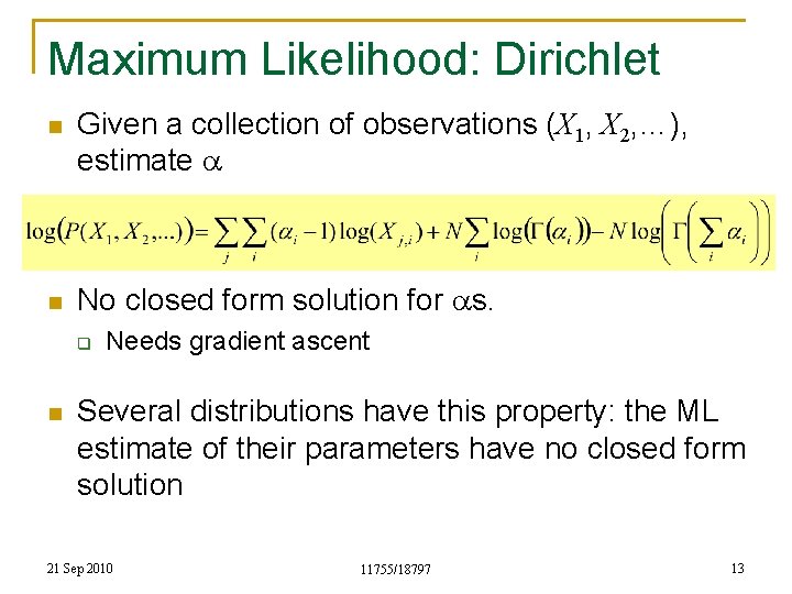
Maximum Likelihood: Dirichlet n n Given a collection of observations (X 1, X 2, …), estimate a No closed form solution for as. q n Needs gradient ascent Several distributions have this property: the ML estimate of their parameters have no closed form solution 21 Sep 2010 11755/18797 13

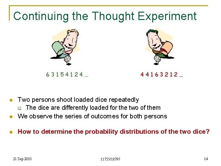
Continuing the Thought Experiment 63154124… 44163212… n Two persons shoot loaded dice repeatedly q The dice are differently loaded for the two of them We observe the series of outcomes for both persons n How to determine the probability distributions of the two dice? n 21 Sep 2010 11755/18797 14

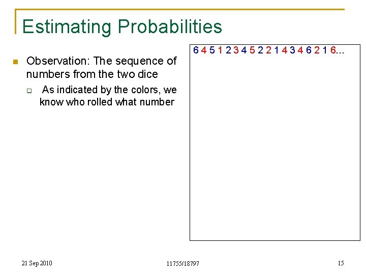
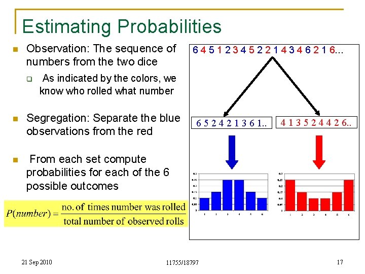
Estimating Probabilities n Observation: The sequence of numbers from the two dice q 6 4 5 1 2 3 4 5 2 2 1 4 3 4 6 2 1 6… As indicated by the colors, we know who rolled what number 21 Sep 2010 11755/18797 15

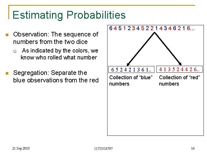
Estimating Probabilities n Observation: The sequence of numbers from the two dice q n 6 4 5 1 2 3 4 5 2 2 1 4 3 4 6 2 1 6… As indicated by the colors, we know who rolled what number Segregation: Separate the blue observations from the red 21 Sep 2010 6 5 2 4 2 1 3 6 1. . 4 1 3 5 2 4 4 2 6. . Collection of “blue” numbers Collection of “red” numbers 11755/18797 16

Estimating Probabilities n Observation: The sequence of numbers from the two dice q 6 4 5 1 2 3 4 5 2 2 1 4 3 4 6 2 1 6… As indicated by the colors, we know who rolled what number n Segregation: Separate the blue observations from the red n From each set compute probabilities for each of the 6 possible outcomes 21 Sep 2010 6 5 2 4 2 1 3 6 1. . 11755/18797 4 1 3 5 2 4 4 2 6. . 17

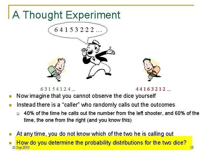
A Thought Experiment 64153222… 44163212… 63154124… n Now imagine that you cannot observe the dice yourself n Instead there is a “caller” who randomly calls out the outcomes q 40% of the time he calls out the number from the left shooter, and 60% of the time, the one from the right (and you know this) n At any time, you do not know which of the two he is calling out n How do you determine the probability distributions for the two dice? 21 Sep 2010 11755/18797 18

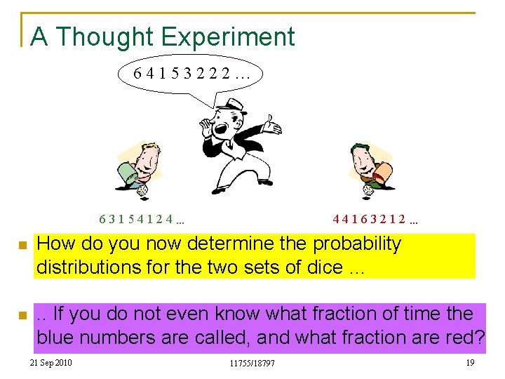
A Thought Experiment 64153222… 44163212… 63154124… n How do you now determine the probability distributions for the two sets of dice … n . . If you do not even know what fraction of time the blue numbers are called, and what fraction are red? 21 Sep 2010 11755/18797 19

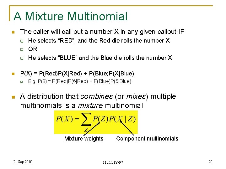
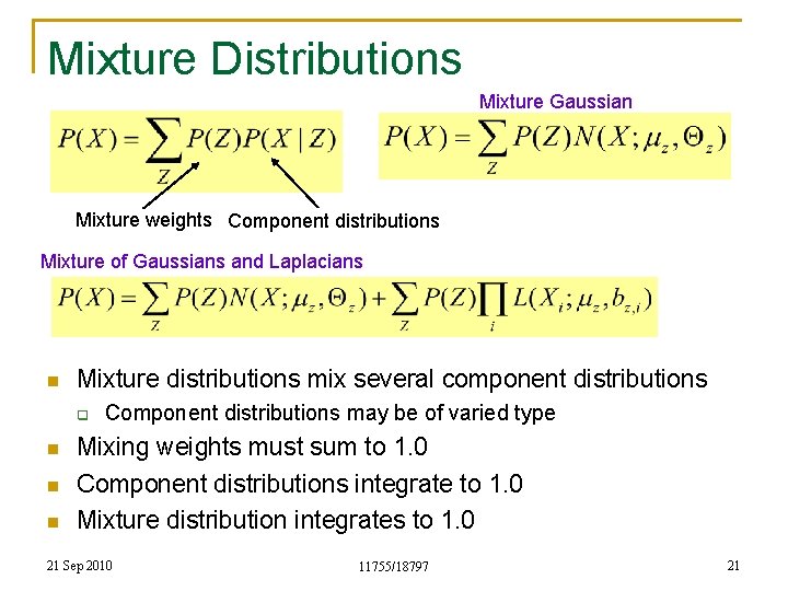
A Mixture Multinomial n The caller will call out a number X in any given callout IF q q q n P(X) = P(Red)P(X|Red) + P(Blue)P(X|Blue) q n He selects “RED”, and the Red die rolls the number X OR He selects “BLUE” and the Blue die rolls the number X E. g. P(6) = P(Red)P(6|Red) + P(Blue)P(6|Blue) A distribution that combines (or mixes) multiple multinomials is a mixture multinomial Mixture weights 21 Sep 2010 Component multinomials 11755/18797 20

Mixture Distributions Mixture Gaussian Mixture weights Component distributions Mixture of Gaussians and Laplacians n Mixture distributions mix several component distributions q n n n Component distributions may be of varied type Mixing weights must sum to 1. 0 Component distributions integrate to 1. 0 Mixture distribution integrates to 1. 0 21 Sep 2010 11755/18797 21

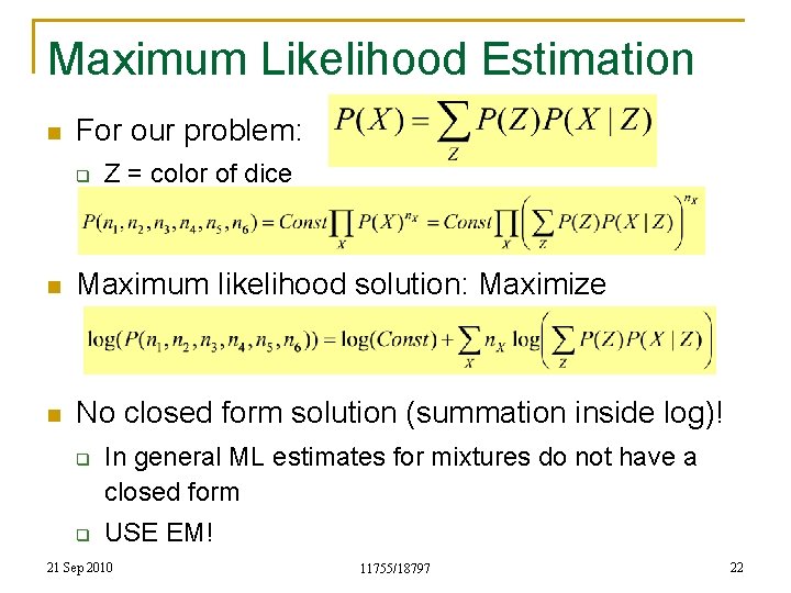
Maximum Likelihood Estimation n For our problem: q Z = color of dice n Maximum likelihood solution: Maximize n No closed form solution (summation inside log)! q q In general ML estimates for mixtures do not have a closed form USE EM! 21 Sep 2010 11755/18797 22

Expectation Maximization n It is possible to estimate all parameters in this setup using the Expectation Maximization (or EM) algorithm n First described in a landmark paper by Dempster, Laird and Rubin q Maximum Likelihood Estimation from incomplete data, via the EM Algorithm, Journal of the Royal Statistical Society, Series B, 1977 n Much work on the algorithm since then n The principles behind the algorithm existed for several years prior to the landmark paper, however. 21 Sep 2010 11755/18797 23

Expectation Maximization n Iterative solution n Get some initial estimates for all parameters q n Dice shooter example: This includes probability distributions for dice AND the probability with which the caller selects the dice Two steps that are iterated: q q Expectation Step: Estimate statistically, the values of unseen variables Maximization Step: Using the estimated values of the unseen variables as truth, estimates of the model parameters 21 Sep 2010 11755/18797 24

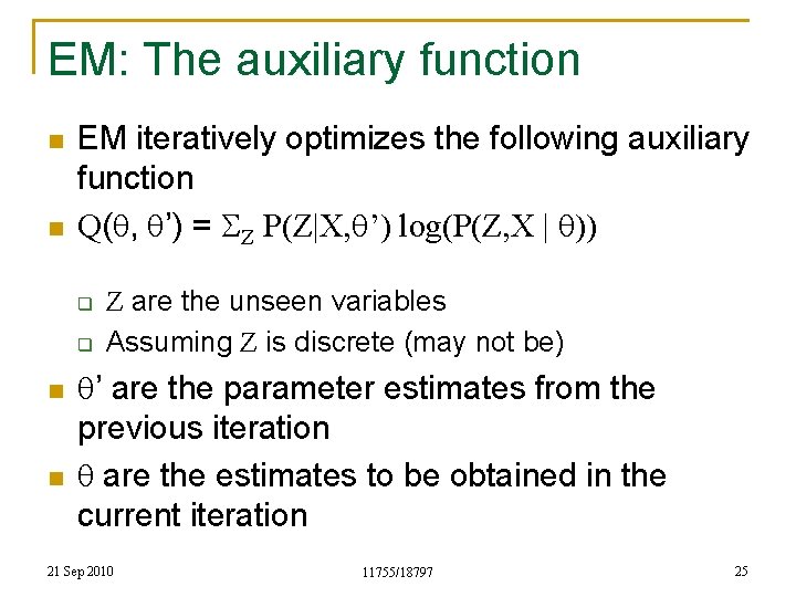
EM: The auxiliary function n n EM iteratively optimizes the following auxiliary function Q(q, q’) = SZ P(Z|X, q’) log(P(Z, X | q)) q q n n Z are the unseen variables Assuming Z is discrete (may not be) q’ are the parameter estimates from the previous iteration q are the estimates to be obtained in the current iteration 21 Sep 2010 11755/18797 25

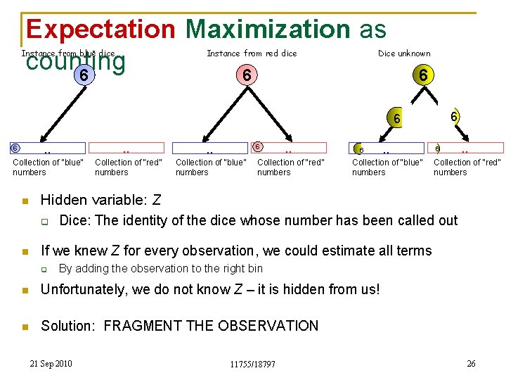
Expectation Maximization as counting 6 6 Instance from blue dice Instance from red dice Dice unknown 6 6 6 . . . Collection of “blue” numbers Collection of “red” numbers Collection of “blue” numbers 6 6 . . Collection of “red” numbers 6 . . Collection of “blue” numbers 6 Collection of “red” numbers n Hidden variable: Z q Dice: The identity of the dice whose number has been called out n If we knew Z for every observation, we could estimate all terms q . . By adding the observation to the right bin n Unfortunately, we do not know Z – it is hidden from us! n Solution: FRAGMENT THE OBSERVATION 21 Sep 2010 11755/18797 26

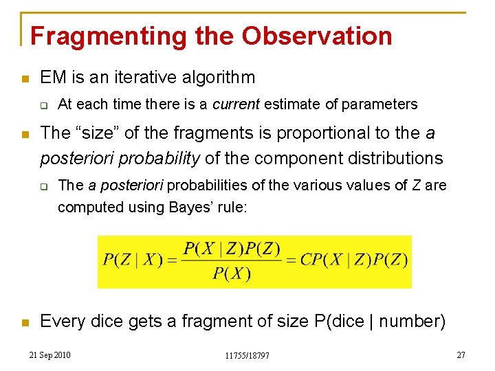
Fragmenting the Observation n EM is an iterative algorithm q n The “size” of the fragments is proportional to the a posteriori probability of the component distributions q n At each time there is a current estimate of parameters The a posteriori probabilities of the various values of Z are computed using Bayes’ rule: Every dice gets a fragment of size P(dice | number) 21 Sep 2010 11755/18797 27

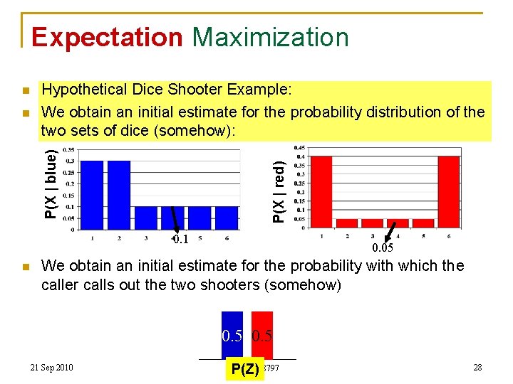
Expectation Maximization n P(X | red) P(X | blue) n Hypothetical Dice Shooter Example: We obtain an initial estimate for the probability distribution of the two sets of dice (somehow): 0. 1 n 0. 05 We obtain an initial estimate for the probability with which the caller calls out the two shooters (somehow) 0. 5 21 Sep 2010 11755/18797 P(Z) 28

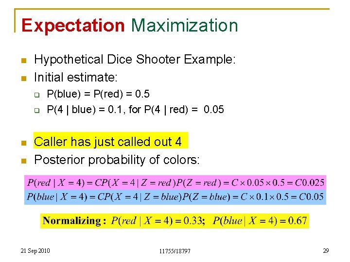
Expectation Maximization n n Hypothetical Dice Shooter Example: Initial estimate: q q n n P(blue) = P(red) = 0. 5 P(4 | blue) = 0. 1, for P(4 | red) = 0. 05 Caller has just called out 4 Posterior probability of colors: 21 Sep 2010 11755/18797 29

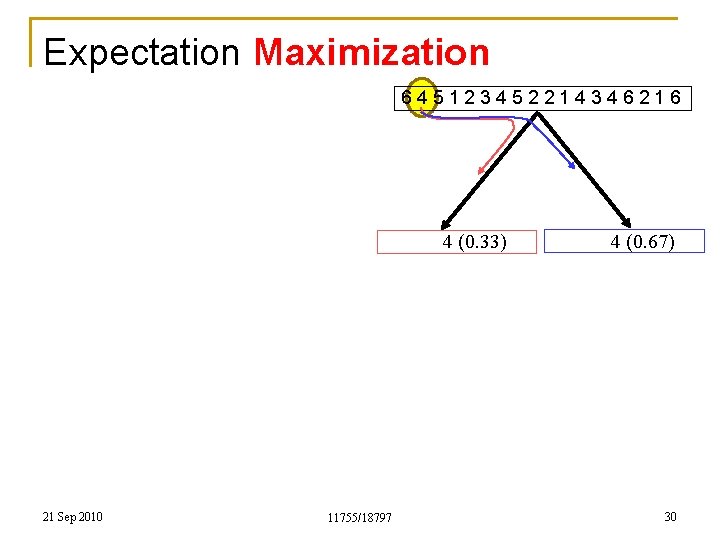
Expectation Maximization 645123452214346216 4 (0. 33) 21 Sep 2010 11755/18797 4 (0. 67) 30

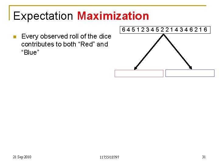
Expectation Maximization n Every observed roll of the dice contributes to both “Red” and “Blue” 21 Sep 2010 11755/18797 645123452214346216 31

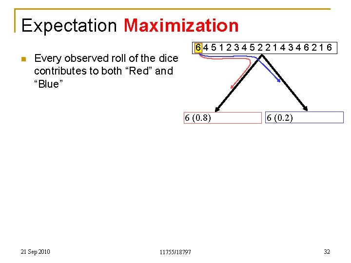
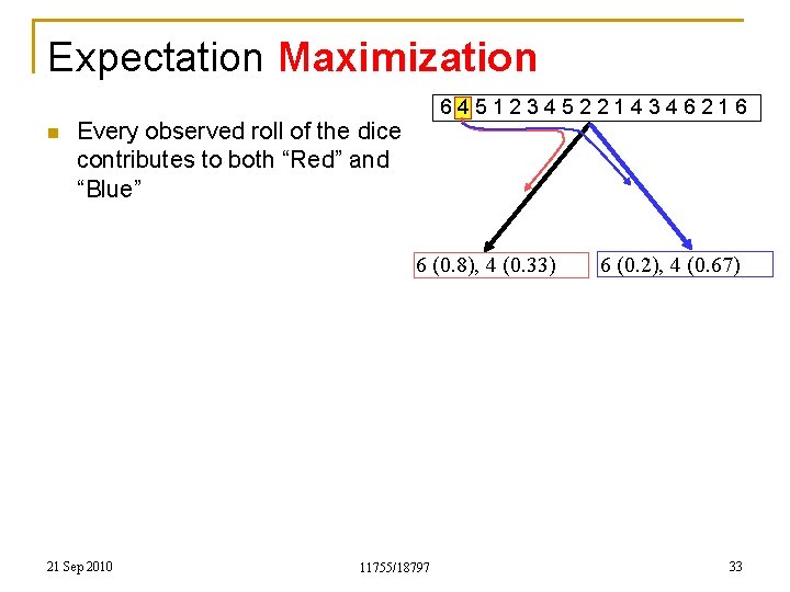
Expectation Maximization n 645123452214346216 Every observed roll of the dice contributes to both “Red” and “Blue” 6 (0. 8) 21 Sep 2010 11755/18797 6 (0. 2) 32

Expectation Maximization n 645123452214346216 Every observed roll of the dice contributes to both “Red” and “Blue” 6 (0. 8), 4 (0. 33) 21 Sep 2010 11755/18797 6 (0. 2), 4 (0. 67) 33

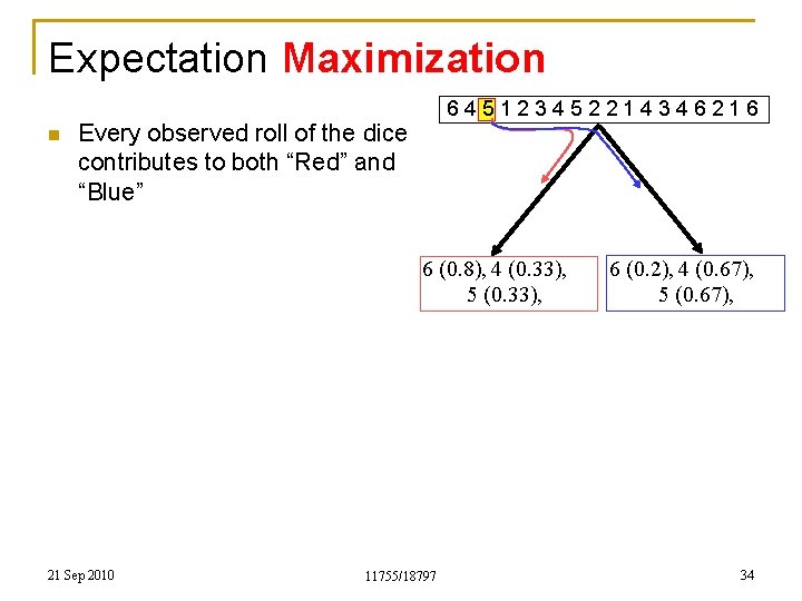
Expectation Maximization n 645123452214346216 Every observed roll of the dice contributes to both “Red” and “Blue” 6 (0. 8), 4 (0. 33), 5 (0. 33), 21 Sep 2010 11755/18797 6 (0. 2), 4 (0. 67), 5 (0. 67), 34

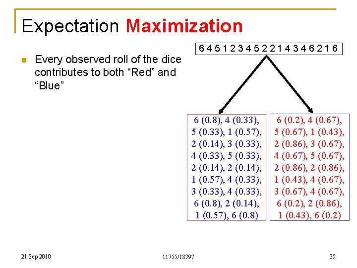
Expectation Maximization n 645123452214346216 Every observed roll of the dice contributes to both “Red” and “Blue” 6 (0. 8), 4 (0. 33), 5 (0. 33), 1 (0. 57), 2 (0. 14), 3 (0. 33), 4 (0. 33), 5 (0. 33), 2 (0. 14), 1 (0. 57), 4 (0. 33), 3 (0. 33), 4 (0. 33), 6 (0. 8), 2 (0. 14), 1 (0. 57), 6 (0. 8) 21 Sep 2010 11755/18797 6 (0. 2), 4 (0. 67), 5 (0. 67), 1 (0. 43), 2 (0. 86), 3 (0. 67), 4 (0. 67), 5 (0. 67), 2 (0. 86), 1 (0. 43), 4 (0. 67), 3 (0. 67), 4 (0. 67), 6 (0. 2), 2 (0. 86), 1 (0. 43), 6 (0. 2) 35

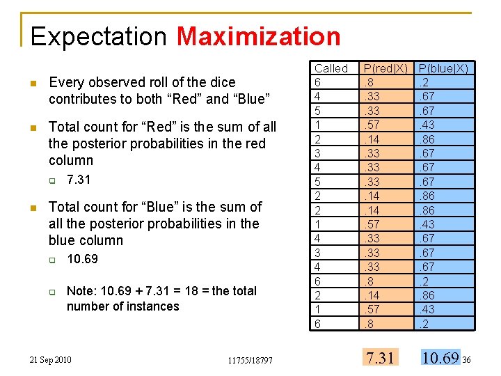
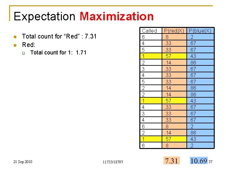
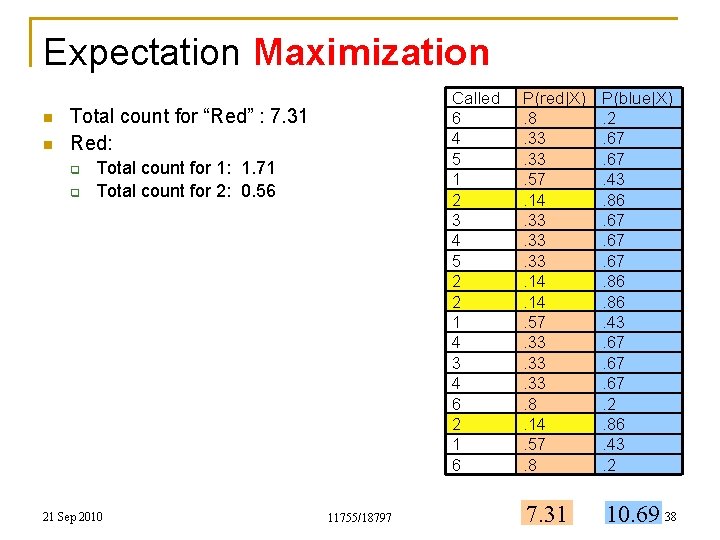
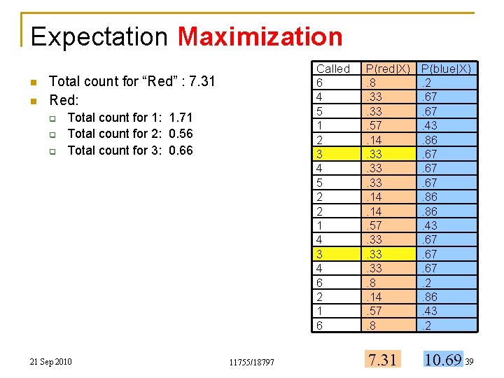
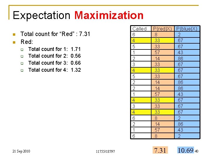
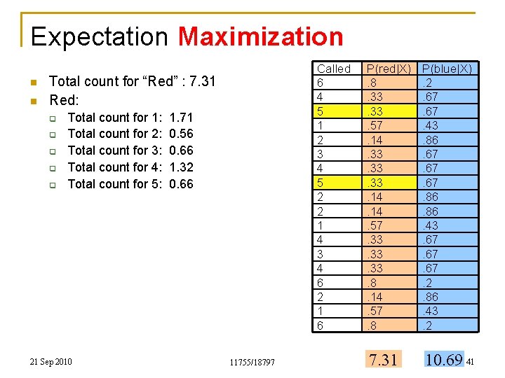
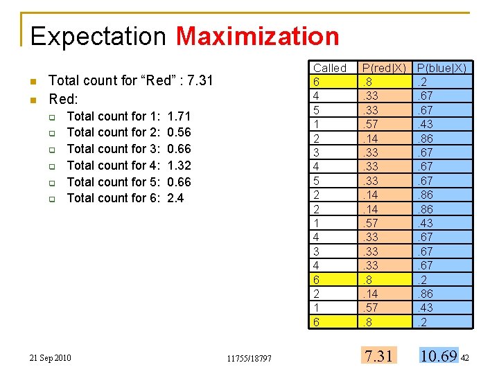
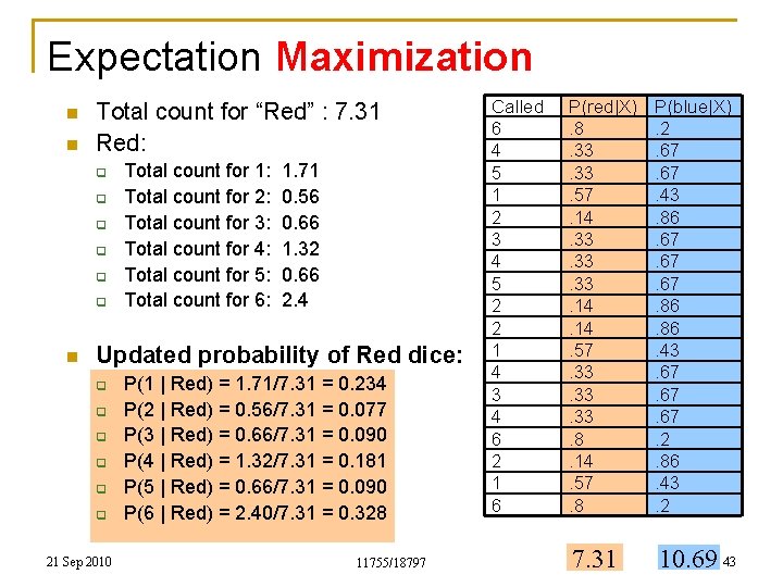
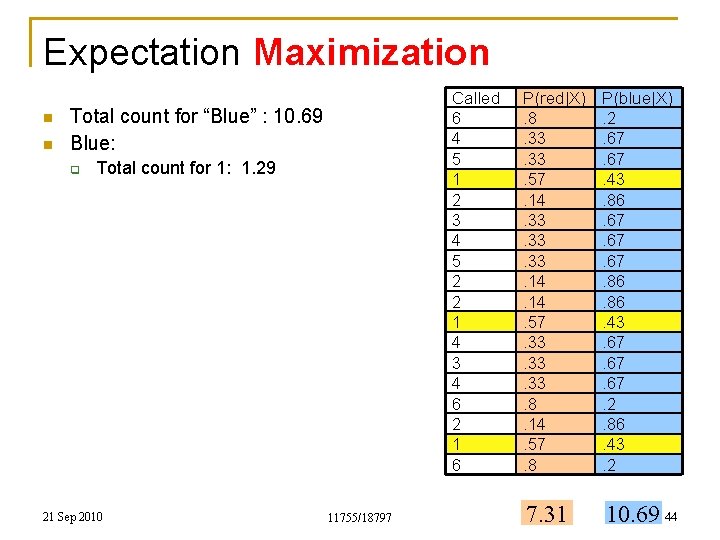
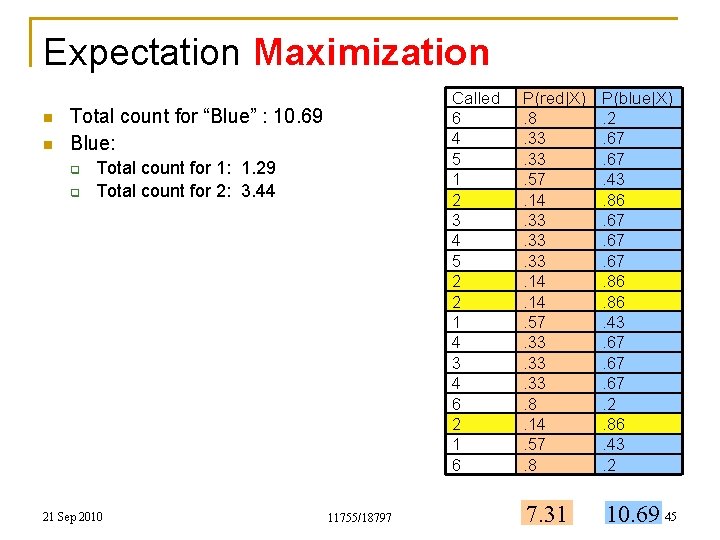
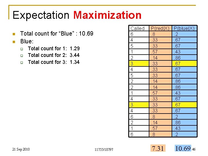
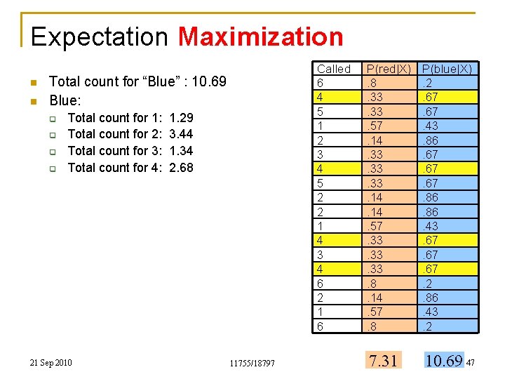
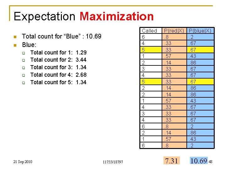
Expectation Maximization n Every observed roll of the dice contributes to both “Red” and “Blue” n Total count for “Red” is the sum of all the posterior probabilities in the red column q n 7. 31 Total count for “Blue” is the sum of all the posterior probabilities in the blue column q q 10. 69 Note: 10. 69 + 7. 31 = 18 = the total number of instances 21 Sep 2010 11755/18797 Called 6 4 5 1 2 3 4 5 2 2 1 4 3 4 6 2 1 6 P(red|X). 8. 33. 57. 14. 33. 33. 14. 57. 33. 33. 8. 14. 57. 8 P(blue|X). 2. 67. 43. 86. 67. 67. 86. 43. 67. 67. 2. 86. 43. 2 7. 31 10. 69 36

Expectation Maximization n n Called 6 4 5 1 2 3 4 5 2 2 1 4 3 4 6 2 1 6 Total count for “Red” : 7. 31 Red: q Total count for 1: 1. 71 21 Sep 2010 11755/18797 P(red|X). 8. 33. 57. 14. 33. 33. 14. 57. 33. 33. 8. 14. 57. 8 P(blue|X). 2. 67. 43. 86. 67. 67. 86. 43. 67. 67. 2. 86. 43. 2 7. 31 10. 69 37

Expectation Maximization n n Called 6 4 5 1 2 3 4 5 2 2 1 4 3 4 6 2 1 6 Total count for “Red” : 7. 31 Red: q q Total count for 1: 1. 71 Total count for 2: 0. 56 21 Sep 2010 11755/18797 P(red|X). 8. 33. 57. 14. 33. 33. 14. 57. 33. 33. 8. 14. 57. 8 P(blue|X). 2. 67. 43. 86. 67. 67. 86. 43. 67. 67. 2. 86. 43. 2 7. 31 10. 69 38

Expectation Maximization n n Called 6 4 5 1 2 3 4 5 2 2 1 4 3 4 6 2 1 6 Total count for “Red” : 7. 31 Red: q q q Total count for 1: 1. 71 Total count for 2: 0. 56 Total count for 3: 0. 66 21 Sep 2010 11755/18797 P(red|X). 8. 33. 57. 14. 33. 33. 14. 57. 33. 33. 8. 14. 57. 8 P(blue|X). 2. 67. 43. 86. 67. 67. 86. 43. 67. 67. 2. 86. 43. 2 7. 31 10. 69 39

Expectation Maximization n n Called 6 4 5 1 2 3 4 5 2 2 1 4 3 4 6 2 1 6 Total count for “Red” : 7. 31 Red: q q Total count for 1: Total count for 2: Total count for 3: Total count for 4: 21 Sep 2010 1. 71 0. 56 0. 66 1. 32 11755/18797 P(red|X). 8. 33. 57. 14. 33. 33. 14. 57. 33. 33. 8. 14. 57. 8 P(blue|X). 2. 67. 43. 86. 67. 67. 86. 43. 67. 67. 2. 86. 43. 2 7. 31 10. 69 40

Expectation Maximization n n Called 6 4 5 1 2 3 4 5 2 2 1 4 3 4 6 2 1 6 Total count for “Red” : 7. 31 Red: q q q Total count for 1: Total count for 2: Total count for 3: Total count for 4: Total count for 5: 21 Sep 2010 1. 71 0. 56 0. 66 1. 32 0. 66 11755/18797 P(red|X). 8. 33. 57. 14. 33. 33. 14. 57. 33. 33. 8. 14. 57. 8 P(blue|X). 2. 67. 43. 86. 67. 67. 86. 43. 67. 67. 2. 86. 43. 2 7. 31 10. 69 41

Expectation Maximization n n Called 6 4 5 1 2 3 4 5 2 2 1 4 3 4 6 2 1 6 Total count for “Red” : 7. 31 Red: q q q Total count for 1: Total count for 2: Total count for 3: Total count for 4: Total count for 5: Total count for 6: 21 Sep 2010 1. 71 0. 56 0. 66 1. 32 0. 66 2. 4 11755/18797 P(red|X). 8. 33. 57. 14. 33. 33. 14. 57. 33. 33. 8. 14. 57. 8 P(blue|X). 2. 67. 43. 86. 67. 67. 86. 43. 67. 67. 2. 86. 43. 2 7. 31 10. 69 42

Expectation Maximization n n Total count for “Red” : 7. 31 Red: q q q n Total count for 1: Total count for 2: Total count for 3: Total count for 4: Total count for 5: Total count for 6: 1. 71 0. 56 0. 66 1. 32 0. 66 2. 4 Updated probability of Red dice: q q q 21 Sep 2010 P(1 | Red) = 1. 71/7. 31 = 0. 234 P(2 | Red) = 0. 56/7. 31 = 0. 077 P(3 | Red) = 0. 66/7. 31 = 0. 090 P(4 | Red) = 1. 32/7. 31 = 0. 181 P(5 | Red) = 0. 66/7. 31 = 0. 090 P(6 | Red) = 2. 40/7. 31 = 0. 328 11755/18797 Called 6 4 5 1 2 3 4 5 2 2 1 4 3 4 6 2 1 6 P(red|X). 8. 33. 57. 14. 33. 33. 14. 57. 33. 33. 8. 14. 57. 8 P(blue|X). 2. 67. 43. 86. 67. 67. 86. 43. 67. 67. 2. 86. 43. 2 7. 31 10. 69 43

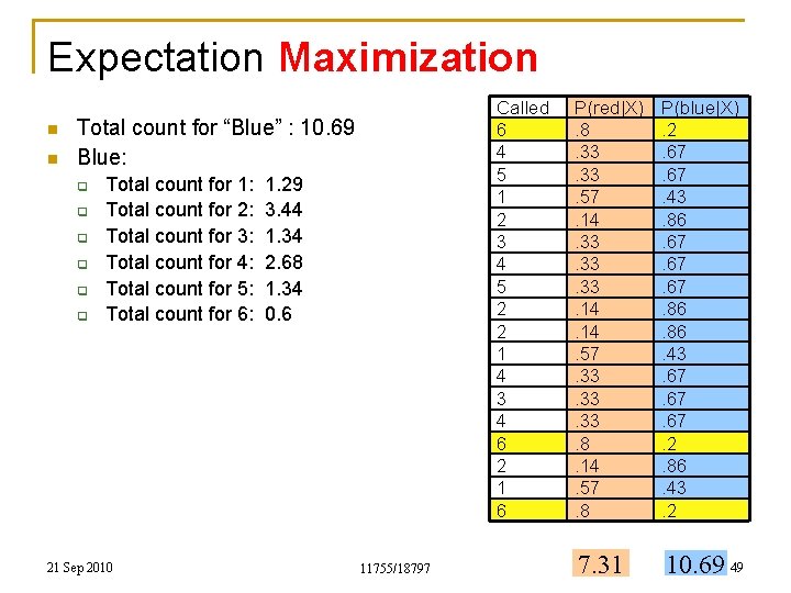
Expectation Maximization n n Called 6 4 5 1 2 3 4 5 2 2 1 4 3 4 6 2 1 6 Total count for “Blue” : 10. 69 Blue: q Total count for 1: 1. 29 21 Sep 2010 11755/18797 P(red|X). 8. 33. 57. 14. 33. 33. 14. 57. 33. 33. 8. 14. 57. 8 P(blue|X). 2. 67. 43. 86. 67. 67. 86. 43. 67. 67. 2. 86. 43. 2 7. 31 10. 69 44

Expectation Maximization n n Called 6 4 5 1 2 3 4 5 2 2 1 4 3 4 6 2 1 6 Total count for “Blue” : 10. 69 Blue: q q Total count for 1: 1. 29 Total count for 2: 3. 44 21 Sep 2010 11755/18797 P(red|X). 8. 33. 57. 14. 33. 33. 14. 57. 33. 33. 8. 14. 57. 8 P(blue|X). 2. 67. 43. 86. 67. 67. 86. 43. 67. 67. 2. 86. 43. 2 7. 31 10. 69 45

Expectation Maximization n n Called 6 4 5 1 2 3 4 5 2 2 1 4 3 4 6 2 1 6 Total count for “Blue” : 10. 69 Blue: q q q Total count for 1: 1. 29 Total count for 2: 3. 44 Total count for 3: 1. 34 21 Sep 2010 11755/18797 P(red|X). 8. 33. 57. 14. 33. 33. 14. 57. 33. 33. 8. 14. 57. 8 P(blue|X). 2. 67. 43. 86. 67. 67. 86. 43. 67. 67. 2. 86. 43. 2 7. 31 10. 69 46

Expectation Maximization n n Called 6 4 5 1 2 3 4 5 2 2 1 4 3 4 6 2 1 6 Total count for “Blue” : 10. 69 Blue: q q Total count for 1: Total count for 2: Total count for 3: Total count for 4: 21 Sep 2010 1. 29 3. 44 1. 34 2. 68 11755/18797 P(red|X). 8. 33. 57. 14. 33. 33. 14. 57. 33. 33. 8. 14. 57. 8 P(blue|X). 2. 67. 43. 86. 67. 67. 86. 43. 67. 67. 2. 86. 43. 2 7. 31 10. 69 47

Expectation Maximization n n Called 6 4 5 1 2 3 4 5 2 2 1 4 3 4 6 2 1 6 Total count for “Blue” : 10. 69 Blue: q q q Total count for 1: Total count for 2: Total count for 3: Total count for 4: Total count for 5: 21 Sep 2010 1. 29 3. 44 1. 34 2. 68 1. 34 11755/18797 P(red|X). 8. 33. 57. 14. 33. 33. 14. 57. 33. 33. 8. 14. 57. 8 P(blue|X). 2. 67. 43. 86. 67. 67. 86. 43. 67. 67. 2. 86. 43. 2 7. 31 10. 69 48

Expectation Maximization n n Called 6 4 5 1 2 3 4 5 2 2 1 4 3 4 6 2 1 6 Total count for “Blue” : 10. 69 Blue: q q q Total count for 1: Total count for 2: Total count for 3: Total count for 4: Total count for 5: Total count for 6: 21 Sep 2010 1. 29 3. 44 1. 34 2. 68 1. 34 0. 6 11755/18797 P(red|X). 8. 33. 57. 14. 33. 33. 14. 57. 33. 33. 8. 14. 57. 8 P(blue|X). 2. 67. 43. 86. 67. 67. 86. 43. 67. 67. 2. 86. 43. 2 7. 31 10. 69 49

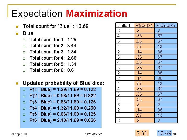
Expectation Maximization n n Total count for “Blue” : 10. 69 Blue: q q q n Total count for 1: Total count for 2: Total count for 3: Total count for 4: Total count for 5: Total count for 6: 1. 29 3. 44 1. 34 2. 68 1. 34 0. 6 Updated probability of Blue dice: q q q 21 Sep 2010 P(1 | Blue) = 1. 29/11. 69 = 0. 122 P(2 | Blue) = 0. 56/11. 69 = 0. 322 P(3 | Blue) = 0. 66/11. 69 = 0. 125 P(4 | Blue) = 1. 32/11. 69 = 0. 250 P(5 | Blue) = 0. 66/11. 69 = 0. 125 P(6 | Blue) = 2. 40/11. 69 = 0. 056 11755/18797 Called 6 4 5 1 2 3 4 5 2 2 1 4 3 4 6 2 1 6 P(red|X). 8. 33. 57. 14. 33. 33. 14. 57. 33. 33. 8. 14. 57. 8 P(blue|X). 2. 67. 43. 86. 67. 67. 86. 43. 67. 67. 2. 86. 43. 2 7. 31 10. 69 50

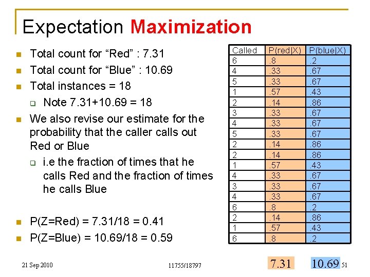
Expectation Maximization n n n Total count for “Red” : 7. 31 Total count for “Blue” : 10. 69 Total instances = 18 q Note 7. 31+10. 69 = 18 We also revise our estimate for the probability that the caller calls out Red or Blue q i. e the fraction of times that he calls Red and the fraction of times he calls Blue P(Z=Red) = 7. 31/18 = 0. 41 P(Z=Blue) = 10. 69/18 = 0. 59 21 Sep 2010 11755/18797 Called 6 4 5 1 2 3 4 5 2 2 1 4 3 4 6 2 1 6 P(red|X). 8. 33. 57. 14. 33. 33. 14. 57. 33. 33. 8. 14. 57. 8 P(blue|X). 2. 67. 43. 86. 67. 67. 86. 43. 67. 67. 2. 86. 43. 2 7. 31 10. 69 51

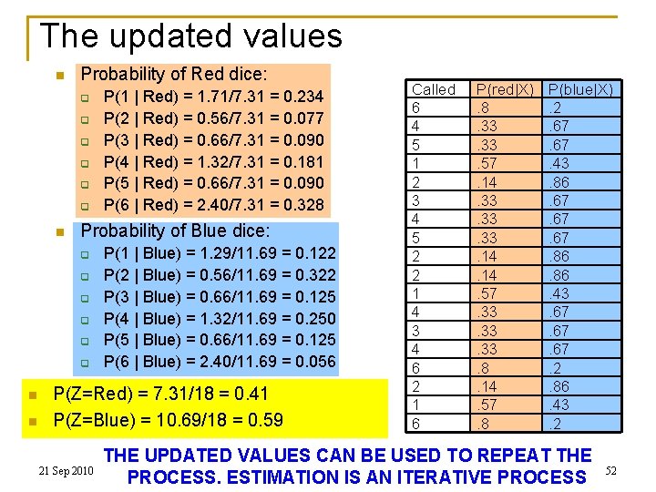
The updated values n Probability of Red dice: q q q n Probability of Blue dice: q q q n n P(1 | Red) = 1. 71/7. 31 = 0. 234 P(2 | Red) = 0. 56/7. 31 = 0. 077 P(3 | Red) = 0. 66/7. 31 = 0. 090 P(4 | Red) = 1. 32/7. 31 = 0. 181 P(5 | Red) = 0. 66/7. 31 = 0. 090 P(6 | Red) = 2. 40/7. 31 = 0. 328 P(1 | Blue) = 1. 29/11. 69 = 0. 122 P(2 | Blue) = 0. 56/11. 69 = 0. 322 P(3 | Blue) = 0. 66/11. 69 = 0. 125 P(4 | Blue) = 1. 32/11. 69 = 0. 250 P(5 | Blue) = 0. 66/11. 69 = 0. 125 P(6 | Blue) = 2. 40/11. 69 = 0. 056 P(Z=Red) = 7. 31/18 = 0. 41 P(Z=Blue) = 10. 69/18 = 0. 59 21 Sep 2010 Called 6 4 5 1 2 3 4 5 2 2 1 4 3 4 6 2 1 6 P(red|X). 8. 33. 57. 14. 33. 33. 14. 57. 33. 33. 8. 14. 57. 8 P(blue|X). 2. 67. 43. 86. 67. 67. 86. 43. 67. 67. 2. 86. 43. 2 THE UPDATED VALUES CAN BE USED TO REPEAT THE 11755/18797 PROCESS. ESTIMATION IS AN ITERATIVE PROCESS 52

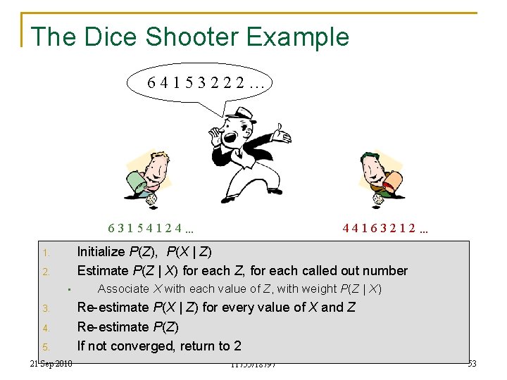
The Dice Shooter Example 64153222… 44163212… 63154124… Initialize P(Z), P(X | Z) Estimate P(Z | X) for each Z, for each called out number 1. 2. • 3. 4. 5. 21 Sep 2010 Associate X with each value of Z, with weight P(Z | X) Re-estimate P(X | Z) for every value of X and Z Re-estimate P(Z) If not converged, return to 2 11755/18797 53

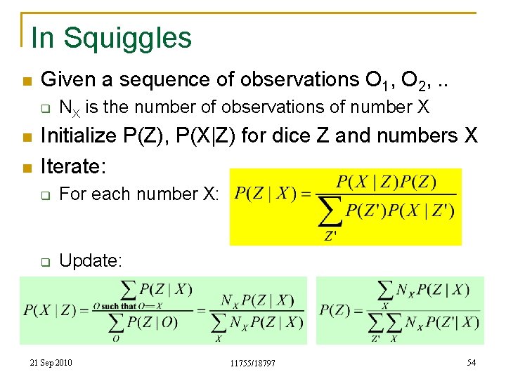
In Squiggles n Given a sequence of observations O 1, O 2, . . q n n NX is the number of observations of number X Initialize P(Z), P(X|Z) for dice Z and numbers X Iterate: q For each number X: q Update: 21 Sep 2010 11755/18797 54

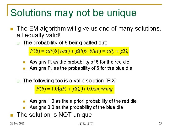
Solutions may not be unique n The EM algorithm will give us one of many solutions, all equally valid! q The probability of 6 being called out: n n q The following too is a valid solution [FIX] n n n Assigns Pr as the probability of 6 for the red die Assigns Pb as the probability of 6 for the blue die Assigns 1. 0 as the a priori probability of the red die Assigns 0. 0 as the probability of the blue die The solution is NOT unique 21 Sep 2010 11755/18797 55

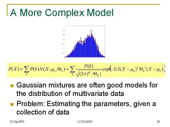
A More Complex Model n n Gaussian mixtures are often good models for the distribution of multivariate data Problem: Estimating the parameters, given a collection of data 21 Sep 2010 11755/18797 56

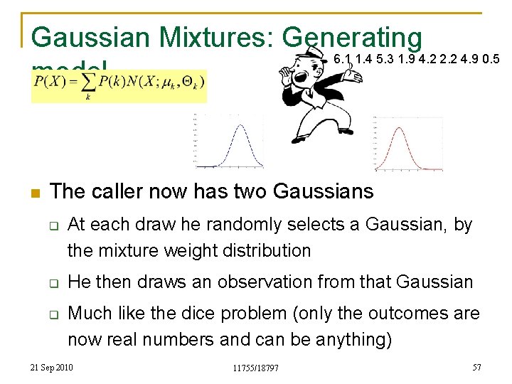
Gaussian Mixtures: Generating 6. 1 1. 4 5. 3 1. 9 4. 2 2. 2 4. 9 0. 5 model n The caller now has two Gaussians q q q At each draw he randomly selects a Gaussian, by the mixture weight distribution He then draws an observation from that Gaussian Much like the dice problem (only the outcomes are now real numbers and can be anything) 21 Sep 2010 11755/18797 57

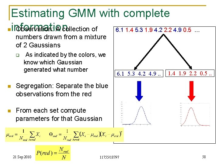
Estimating GMM with complete information Observation: A collection of 6. 1 1. 4 5. 3 1. 9 4. 2 2. 2 4. 9 0. 5 … n numbers drawn from a mixture of 2 Gaussians q As indicated by the colors, we know which Gaussian generated what number n Segregation: Separate the blue observations from the red n From each set compute parameters for that Gaussian 21 Sep 2010 6. 1 5. 3 4. 2 4. 9. . 11755/18797 1. 4 1. 9 2. 2 0. 5. . 58

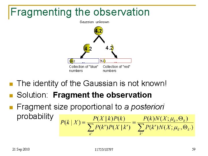
Fragmenting the observation Gaussian unknown 4. 2 . . 4. 2 Collection of “blue” numbers n n n . . Collection of “red” numbers The identity of the Gaussian is not known! Solution: Fragment the observation Fragment size proportional to a posteriori probability 21 Sep 2010 11755/18797 59

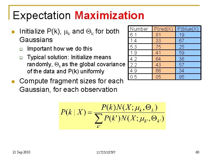
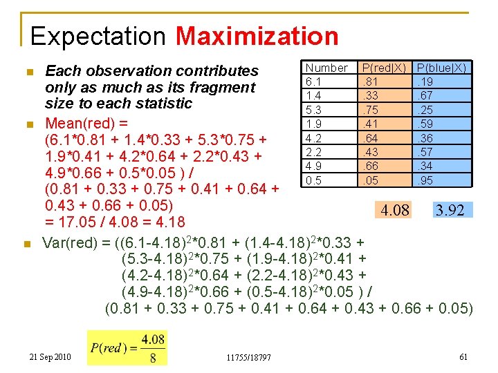
Expectation Maximization n q q n Number 6. 1 1. 4 5. 3 Important how we do this 1. 9 Typical solution: Initialize means 4. 2 randomly, Qk as the global covariance 2. 2 4. 9 of the data and P(k) uniformly 0. 5 Initialize P(k), mk and Qk for both Gaussians Compute fragment sizes for each Gaussian, for each observation 21 Sep 2010 11755/18797 P(red|X). 81. 33. 75. 41. 64. 43. 66. 05 P(blue|X). 19. 67. 25. 59. 36. 57. 34. 95 60

Expectation Maximization n Number P(red|X) P(blue|X) Each observation contributes 6. 1. 81. 19 only as much as its fragment 1. 4. 33. 67 size to each statistic 5. 3. 75. 25 1. 9. 41. 59 Mean(red) = 4. 2. 64. 36 (6. 1*0. 81 + 1. 4*0. 33 + 5. 3*0. 75 + 2. 2. 43. 57 1. 9*0. 41 + 4. 2*0. 64 + 2. 2*0. 43 + 4. 9. 66. 34 4. 9*0. 66 + 0. 5*0. 05 ) / 0. 5. 05. 95 (0. 81 + 0. 33 + 0. 75 + 0. 41 + 0. 64 + 0. 43 + 0. 66 + 0. 05) 4. 08 3. 92 = 17. 05 / 4. 08 = 4. 18 Var(red) = ((6. 1 -4. 18)2*0. 81 + (1. 4 -4. 18)2*0. 33 + (5. 3 -4. 18)2*0. 75 + (1. 9 -4. 18)2*0. 41 + (4. 2 -4. 18)2*0. 64 + (2. 2 -4. 18)2*0. 43 + (4. 9 -4. 18)2*0. 66 + (0. 5 -4. 18)2*0. 05 ) / (0. 81 + 0. 33 + 0. 75 + 0. 41 + 0. 64 + 0. 43 + 0. 66 + 0. 05) 21 Sep 2010 11755/18797 61

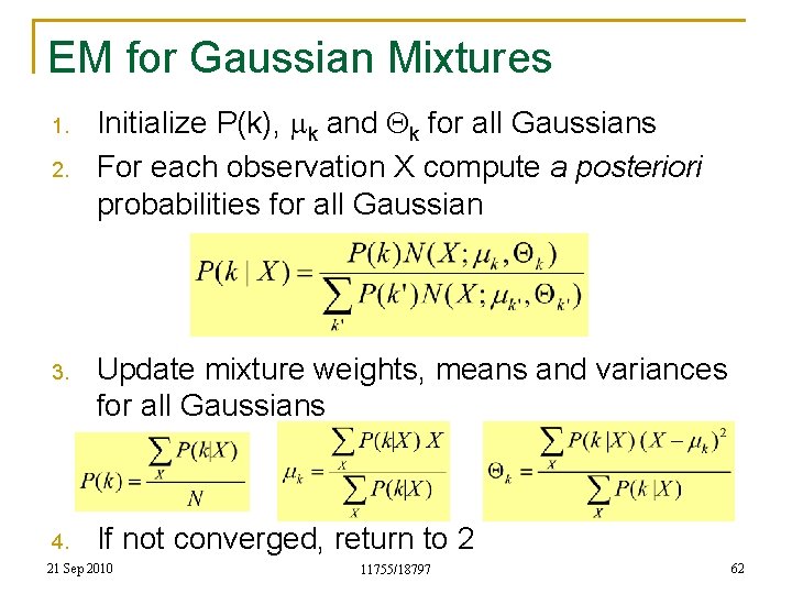
EM for Gaussian Mixtures 1. 2. Initialize P(k), mk and Qk for all Gaussians For each observation X compute a posteriori probabilities for all Gaussian 3. Update mixture weights, means and variances for all Gaussians 4. If not converged, return to 2 21 Sep 2010 11755/18797 62

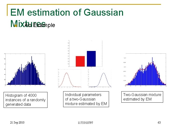
EM estimation of Gaussian n An Example Mixtures Histogram of 4000 instances of a randomly generated data 21 Sep 2010 Individual parameters of a two-Gaussian mixture estimated by EM 11755/18797 Two-Gaussian mixture estimated by EM 63

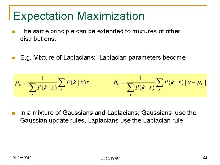
Expectation Maximization n The same principle can be extended to mixtures of other distributions. n E. g. Mixture of Laplacians: Laplacian parameters become n In a mixture of Gaussians and Laplacians, Gaussians use the Gaussian update rules, Laplacians use the Laplacian rule 21 Sep 2010 11755/18797 64

Expectation Maximization n The EM algorithm is used whenever proper statistical analysis of a phenomenon requires the knowledge of a hidden or missing variable (or a set of hidden/missing variables) q n The hidden variable is often called a “latent” variable Some examples: q Estimating mixtures of distributions n q q Only data are observed. The individual distributions and mixing proportions must both be learnt. Estimating the distribution of data, when some attributes are missing Estimating the dynamics of a system, based only on observations that may be a complex function of system state 21 Sep 2010 11755/18797 65

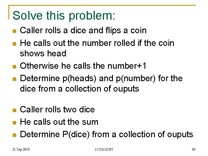
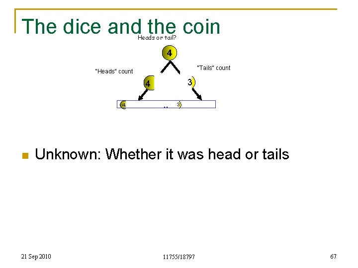
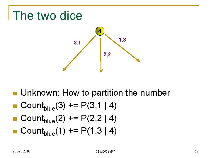
Solve this problem: n n n n Caller rolls a dice and flips a coin He calls out the number rolled if the coin shows head Otherwise he calls the number+1 Determine p(heads) and p(number) for the dice from a collection of ouputs Caller rolls two dice He calls out the sum Determine P(dice) from a collection of ouputs 21 Sep 2010 11755/18797 66

The dice and the coin Heads or tail? 4 “Tails” count “Heads” count 3 4 4. n . . 3 Unknown: Whether it was head or tails 21 Sep 2010 11755/18797 67

The two dice 4 1, 3 3, 1 2, 2 n n Unknown: How to partition the number Countblue(3) += P(3, 1 | 4) Countblue(2) += P(2, 2 | 4) Countblue(1) += P(1, 3 | 4) 21 Sep 2010 11755/18797 68

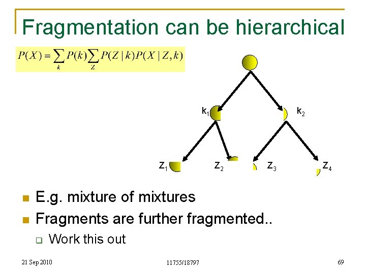
Fragmentation can be hierarchical k 1 Z 1 n n k 2 Z 3 Z 4 E. g. mixture of mixtures Fragments are further fragmented. . q Work this out 21 Sep 2010 11755/18797 69

More later n n Will see a couple of other instances of the use of EM Work out HMM training q q q Assume state output distributions are multinomials Assume they are Gaussian Assume Gaussian mixtures 21 Sep 2010 11755/18797 70