1005 ICT lecture 5 Complexity Analysis Sorting Searching

1005 ICT: : lecture 5 Complexity Analysis, Sorting & Searching 1 11/2/2020 Written by Rob Baltrusch, some parts adapted from Sun.

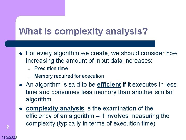
What is complexity analysis? l For every algorithm we create, we should consider how increasing the amount of input data increases: – – l l 2 11/2/2020 Execution time Memory required for execution An algorithm is said to be efficient if it executes in less time and consumes less memory than another similar algorithm complexity analysis is the examination of the efficiency of an algorithm – it involves measuring the complexity (typically in terms of execution time)

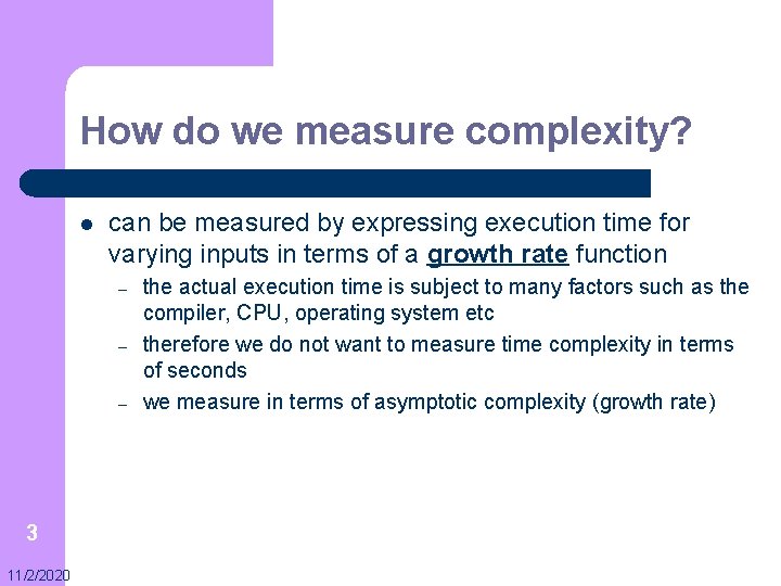
How do we measure complexity? l can be measured by expressing execution time for varying inputs in terms of a growth rate function – – – 3 11/2/2020 the actual execution time is subject to many factors such as the compiler, CPU, operating system etc therefore we do not want to measure time complexity in terms of seconds we measure in terms of asymptotic complexity (growth rate)

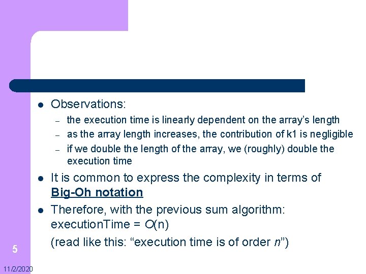
l For example, consider the simple sum algorithm below int sum(int[] a){ int result = 0; for(int i = 0; i < a. length; i++){ result += a[i]; } return result; } l execution. Time //assignment: time = t 1 //loop: time = t 2 //assignment: time = t 3 //return: time = t 4 = t 1 + n * (t 2 + t 3) + t 4 = k 1 + n * k 2 = n * k 2 where k 1 and k 2 are method dependent constants since statements are done in constant time 4 11/2/2020

l Observations: – – – l l 5 11/2/2020 the execution time is linearly dependent on the array’s length as the array length increases, the contribution of k 1 is negligible if we double the length of the array, we (roughly) double the execution time It is common to express the complexity in terms of Big-Oh notation Therefore, with the previous sum algorithm: execution. Time = O(n) (read like this: “execution time is of order n”)

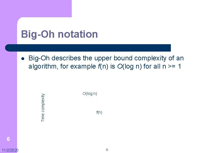
Big-Oh notation Big-Oh describes the upper bound complexity of an algorithm, for example f(n) is O(log n) for all n >= 1 Time complexity l O(log n) f(n) 6 11/2/2020 n

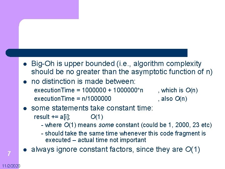
l l Big-Oh is upper bounded (i. e. , algorithm complexity should be no greater than the asymptotic function of n) no distinction is made between: execution. Time = 1000000 + 1000000*n execution. Time = n/1000000 l , which is O(n) , also O(n) some statements take constant time: result += a[i]; O(1) - where O(1) means some constant (could be 1, 2000, 23 etc) - should take the same time whenever this code fragment is executed – actual time not important 7 11/2/2020 l always ignore constant factors, since they are O(1)

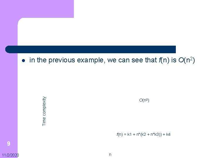
int process. Array(int[] a){ int result = 0; for(int i = 0; i < a. length; i++){ for(int j = 0; j < a. length; j++){ result += a[i] * a[j]; } } return result; } execution. Time = t 1 + n * (t 2 + n * (t 3 + t 4)) + t 5 = k 1 + n * (k 2 + n * k 3)) + k 4 =n*n = O(n 2) 8 11/2/2020 Therefore, the algorithm is of order n 2 //t 1 //t 2 //t 3 //t 4 //t 5

in the previous example, we can see that f(n) is O(n 2) Time complexity l O(n 2) f(n) = k 1 + n*(k 2 + n*k 3)) + k 4 9 11/2/2020 n

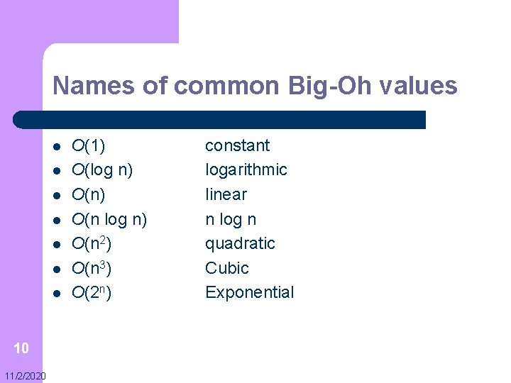
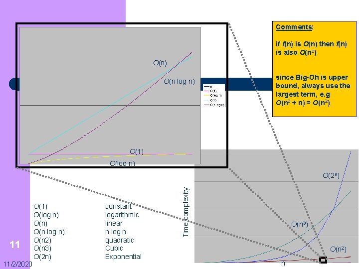
Names of common Big-Oh values l l l l 10 11/2/2020 O(1) O(log n) O(n 2) O(n 3) O(2 n) constant logarithmic linear n log n quadratic Cubic Exponential

Comments: if f(n) is O(n) then f(n) is also O(n 2) O(n log n) since Big-Oh is upper bound, always use the largest term, e. g O(n 2 + n) = O(n 2) O(1) O(log n) 11 11/2/2020 O(1) O(log n) O(n 2) O(n 3) O(2 n) constant logarithmic linear n log n quadratic Cubic Exponential Time complexity O(2 n) O(n 3) O(n 2) n

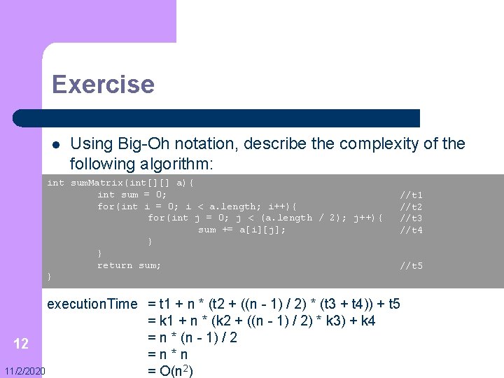
Exercise l Using Big-Oh notation, describe the complexity of the following algorithm: int sum. Matrix(int[][] a){ int sum = 0; for(int i = 0; i < a. length; i++){ for(int j = 0; j < (a. length / 2); j++){ sum += a[i][j]; } } return sum; } //t 1 //t 2 //t 3 //t 4 //t 5 execution. Time = t 1 + n * (t 2 + ((n - 1) / 2) * (t 3 + t 4)) + t 5 = k 1 + n * (k 2 + ((n - 1) / 2) * k 3) + k 4 = n * (n - 1) / 2 12 =n*n 11/2/2020 = O(n 2)

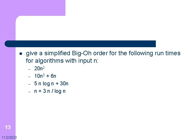
l give a simplified Big-Oh order for the following run times for algorithms with input n: – – 13 11/2/2020 20 n 2 10 n 3 + 6 n 5 n log n + 30 n n + 3 n / log n

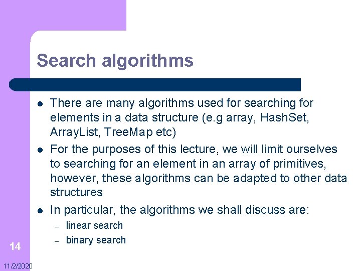
Search algorithms l l l There are many algorithms used for searching for elements in a data structure (e. g array, Hash. Set, Array. List, Tree. Map etc) For the purposes of this lecture, we will limit ourselves to searching for an element in an array of primitives, however, these algorithms can be adapted to other data structures In particular, the algorithms we shall discuss are: – 14 11/2/2020 – linear search binary search

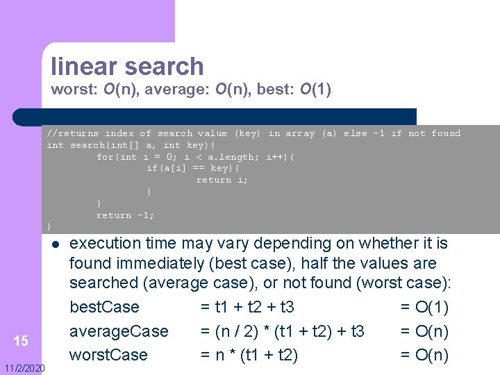
linear search worst: O(n), average: O(n), best: O(1) //returns index of search value (key) in array (a) else -1 if not found int search(int[] a, int key){ for(int i = 0; i < a. length; i++){ if(a[i] == key){ return i; } } return -1; } l 15 11/2/2020 execution time may vary depending on whether it is found immediately (best case), half the values are searched (average case), or not found (worst case): best. Case = t 1 + t 2 + t 3 = O(1) average. Case = (n / 2) * (t 1 + t 2) + t 3 = O(n) worst. Case = n * (t 1 + t 2) = O(n)

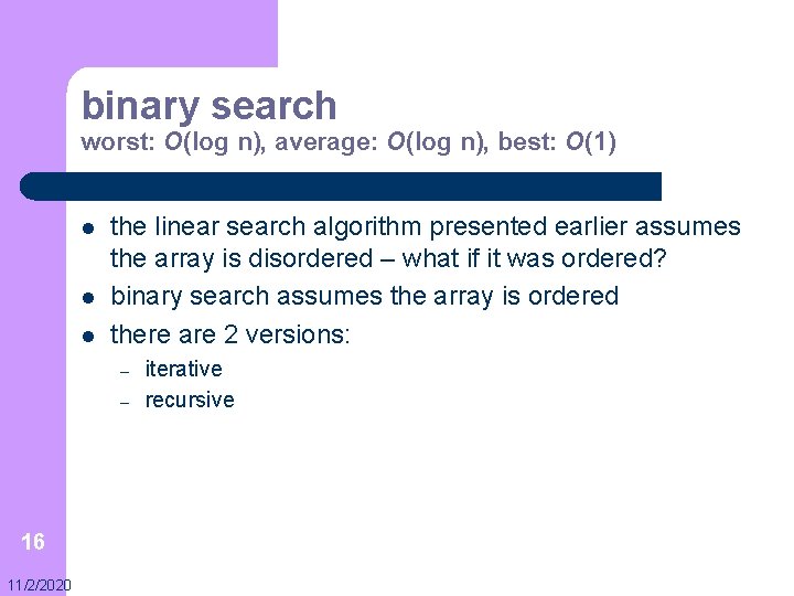
binary search worst: O(log n), average: O(log n), best: O(1) l l l the linear search algorithm presented earlier assumes the array is disordered – what if it was ordered? binary search assumes the array is ordered there are 2 versions: – – 16 11/2/2020 iterative recursive

l iterative binary search //returns index of search value (key) in array (a) else -1 if not found //pre: array a is in ascending order int search(int[] a, int key){ int left, middle, right; left = 0; right = a. length; while(left <= right){ middle = (left + right) / 2; if(a[middle] == key){ return middle; }else if(a[middle] < key){ left = middle + 1; }else{ right = middle – 1; } } 17 return -1; 11/2/2020 }

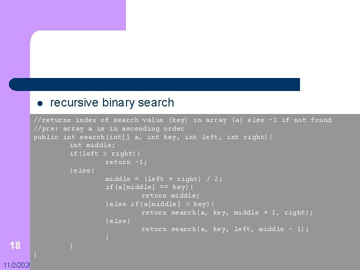
l 18 11/2/2020 recursive binary search //returns index of search value (key) in array (a) else -1 if not found //pre: array a is in ascending order public int search(int[] a, int key, int left, int right){ int middle; if(left > right){ return -1; }else{ middle = (left + right) / 2; if(a[middle] == key){ return middle; }else if(a[middle] < key){ return search(a, key, middle + 1, right); }else{ return search(a, key, left, middle - 1); } } }

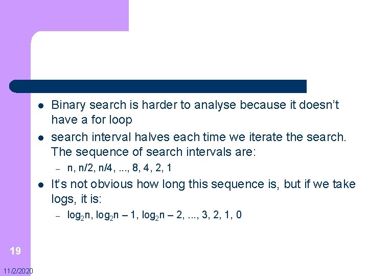
l l Binary search is harder to analyse because it doesn’t have a for loop search interval halves each time we iterate the search. The sequence of search intervals are: – l It’s not obvious how long this sequence is, but if we take logs, it is: – 19 11/2/2020 n, n/2, n/4, . . . , 8, 4, 2, 1 log 2 n, log 2 n – 1, log 2 n – 2, . . . , 3, 2, 1, 0

l l l 20 11/2/2020 Since the second sequence decrements by 1 each time down to 0, its length must be log 2 n + 1. It takes only constant time to do each test of binary search, so the total running time is just the number of times that we iterate, which is log 2 n + 1 Therefore binary search is an O(log 2 n) algorithm Since the base of the log doesn’t matter in an asymptotic bound, we can write that binary search is O(log n)

Sort algorithms l l again, we will limit ourselves to sorting an array of primitives, however, these algorithms can be adapted to other data structures The sort algorithms we shall discuss are: – – – 21 11/2/2020 bubble sort selection sort insertion sort merge sort quick sort

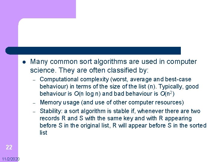
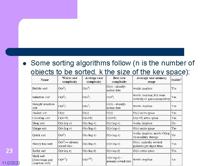
l Many common sort algorithms are used in computer science. They are often classified by: – – – 22 11/2/2020 Computational complexity (worst, average and best-case behaviour) in terms of the size of the list (n). Typically, good behaviour is O(n log n) and bad behaviour is O(n 2) Memory usage (and use of other computer resources) Stability: a sort algorithm is stable if, whenever there are two records R and S with the same key and with R appearing before S in the original list, R will appear before S in the sorted list

l 23 11/2/2020 Some sorting algorithms follow (n is the number of objects to be sorted, k the size of the key space):

bubble sort worst: O(n 2), average: O(n 2), best: O(n) l Bubble sort is a simple sorting algorithm – – 24 11/2/2020 It takes a lot of passes through the list to be sorted, comparing two items at a time, swapping these two items in the correct order if necessary Bubble sort gets its name from the fact that the items that belong at the top of the list gradually "float" up there

l Bubble sort needs O(n 2) comparisons to sort n items and can sort in place. – l It is essentially equivalent to insertion sort - it compares and swaps the same pairs of elements, just in a different order – 25 11/2/2020 It is one of the simplest sorting algorithms to understand but is generally too inefficient for serious work sorting large numbers of elements Naive implementations of bubble sort (like those in the following slides) usually perform badly on already-sorted lists (O(n 2)), while insertion sort needs only O(n) operations in this case

l improving efficiency: – 26 11/2/2020 It is possible to reduce the best case complexity to O(n) if a flag is used to denote whether any swaps were necessary during the first run of the inner loop. In this case, no swaps would indicate an already sorted list

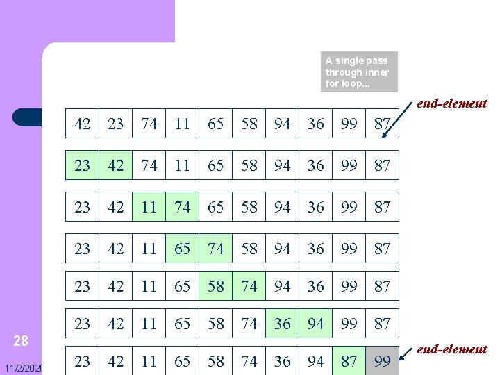
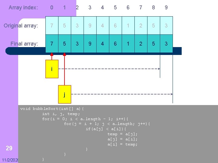
l The bubble sort algorithm is: – – 27 11/2/2020 1. Compare adjacent elements. If the first is greater than the second, swap them 2. Do this for each pair of adjacent elements, starting with the first two and ending with the last two. At this point the last element should be the greatest 3. Repeat the steps for all elements except the last one 4. Keep repeating for one fewer elements each time, until you have no more pairs to compare

A single pass through inner for loop. . . end-element 42 23 74 11 65 58 94 36 99 87 23 42 11 74 65 58 94 36 99 87 23 42 11 65 74 58 94 36 99 87 23 42 11 65 58 74 36 94 99 87 28 11/2/2020 23 42 11 65 58 74 36 94 87 99 end-element

Array index: 0 1 2 3 4 5 6 7 8 9 Original array: 7 5 3 9 4 6 1 2 5 3 Final array: 7 5 3 9 4 6 1 2 5 3 i j void bubble. Sort(int[] a){ int i, j, temp; for(i = 0; i < a. length – 1; i++){ for(j = i + 1; j < a. length; j++){ if(a[j] < a[i]){ temp = a[j]; a[j] = a[i]; a[i] = temp; 29 } } } 11/2/2020

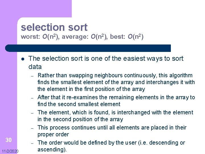
selection sort worst: O(n 2), average: O(n 2), best: O(n 2) l The selection sort is one of the easiest ways to sort data – – 30 11/2/2020 – Rather than swapping neighbours continuously, this algorithm finds the smallest element of the array and interchanges it with the element in the first position of the array After that it re-examines the remaining elements in the array to find the second smallest element The element, which is found, is interchanged with the element in the second position of the array This process continues until all elements are placed in their proper order The order would be defined by the user (i. e. descending or ascending).

l For each position in the array: – – – 31 11/2/2020 1. Scan the unsorted part of the data 2. Select the smallest value 3. Switch the smallest value with the first value in the unsorted part of the data

32 11/2/2020 void selection. Sort(int[] a){ for (int i = 0; i < a. length - 1; i++){ int min. Index = i; for (int j = i + 1; j < a. length; j++){ if (a[j] < a[min. Index]){ min. Index = j; } } if (min. Index != i){ int temp = a[i]; a[i] = a[min. Index]; a[min. Index] = temp; } } }

l l 33 11/2/2020 Selection sort is O(n 2 ) in the best, worst, and expected cases The selection sort is easy to understand this makes it easy to implement the algorithm correctly and thus makes the sorting procedure easy to write

l However, there are some reasons why programmers refrain from using this algorithm: – – 34 11/2/2020 1. This program's performance of O(n 2 ) would become quite slow on large amounts of data 2. At present many application databases have sorted lists of data and these lists are updated on a regular basis. Most times these databases are, for the most part, in order. An ideal method would be able to recognize this fact and would work only on the unsorted items. The selection sort is unable to do this

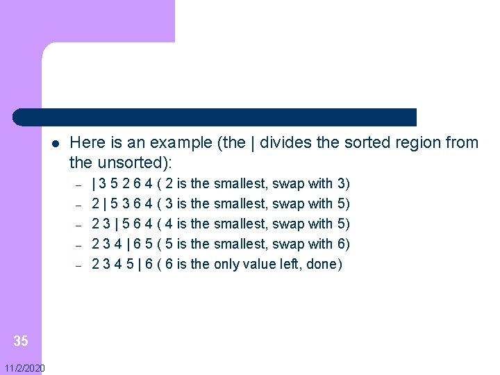
l Here is an example (the | divides the sorted region from the unsorted): – – – 35 11/2/2020 | 3 5 2 6 4 ( 2 is the smallest, swap with 3) 2 | 5 3 6 4 ( 3 is the smallest, swap with 5) 2 3 | 5 6 4 ( 4 is the smallest, swap with 5) 2 3 4 | 6 5 ( 5 is the smallest, swap with 6) 2 3 4 5 | 6 ( 6 is the only value left, done)

insertion sort worst: O(n 2), average: O(n 2), best: O(n) l Insertion sort is a simple sort algorithm where the result is built up one entry at a time – – 36 11/2/2020 In abstract terms, each iteration of an insertion sort removes an element from the input data, inserting it at the correct position in the already sorted list, until no elements are left in the input The choice of which element to remove from the input is arbitrary

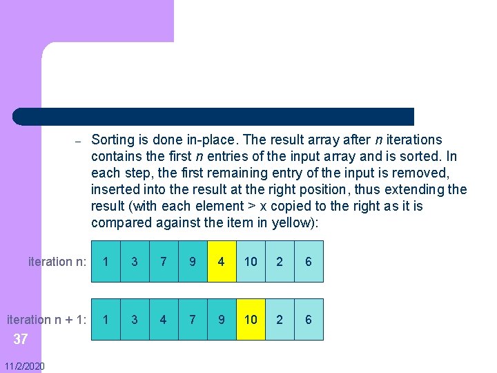
– Sorting is done in-place. The result array after n iterations contains the first n entries of the input array and is sorted. In each step, the first remaining entry of the input is removed, inserted into the result at the right position, thus extending the result (with each element > x copied to the right as it is compared against the item in yellow): iteration n: 1 3 7 9 4 10 2 6 iteration n + 1: 1 3 4 7 9 10 2 6 37 11/2/2020

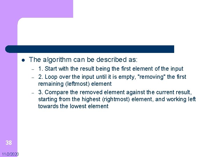
l The algorithm can be described as: – – – 38 11/2/2020 1. Start with the result being the first element of the input 2. Loop over the input until it is empty, "removing" the first remaining (leftmost) element 3. Compare the removed element against the current result, starting from the highest (rightmost) element, and working left towards the lowest element

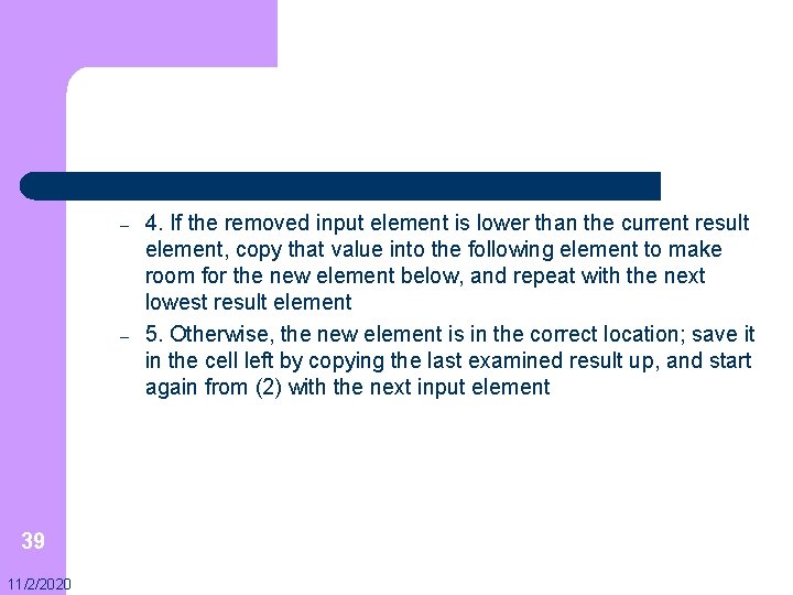
– – 39 11/2/2020 4. If the removed input element is lower than the current result element, copy that value into the following element to make room for the new element below, and repeat with the next lowest result element 5. Otherwise, the new element is in the correct location; save it in the cell left by copying the last examined result up, and start again from (2) with the next input element

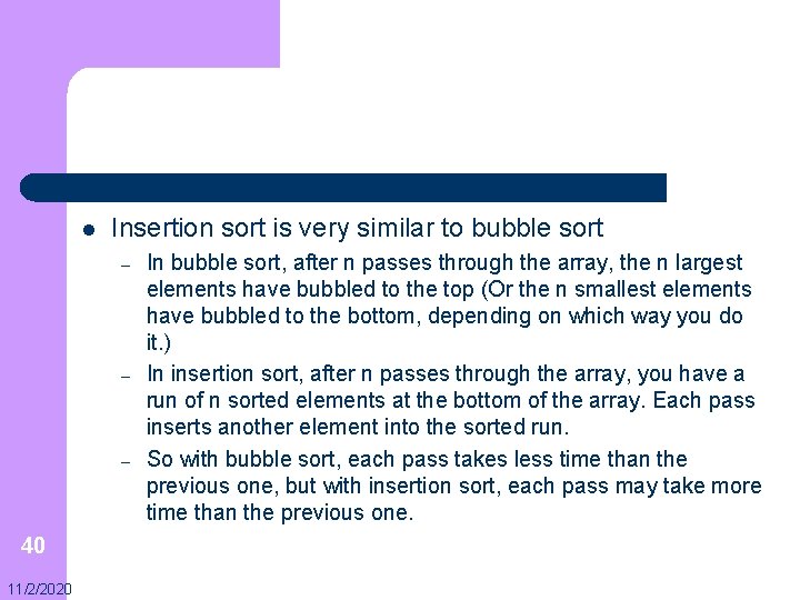
l Insertion sort is very similar to bubble sort – – – 40 11/2/2020 In bubble sort, after n passes through the array, the n largest elements have bubbled to the top (Or the n smallest elements have bubbled to the bottom, depending on which way you do it. ) In insertion sort, after n passes through the array, you have a run of n sorted elements at the bottom of the array. Each pass inserts another element into the sorted run. So with bubble sort, each pass takes less time than the previous one, but with insertion sort, each pass may take more time than the previous one.

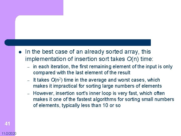
l In the best case of an already sorted array, this implementation of insertion sort takes O(n) time: – – – 41 11/2/2020 in each iteration, the first remaining element of the input is only compared with the last element of the result It takes O(n 2) time in the average and worst cases, which makes it impractical for sorting large numbers of elements However, insertion sort's inner loop is very fast, which often makes it one of the fastest algorithms for sorting small numbers of elements, typically less than 10 or so

void insertion. Sort(int[] a){ for (int i = 1; i < a. length; i++){ int item. To. Insert = a[i]; int j = i - 1; while (j >= 0){ if (item. To. Insert < a[j]){ a[j + 1] = a[j]; j--; }else{ break; } a[j + 1] = item. To. Insert; } } 42 11/2/2020

merge sort worst: O(n log n), average: O(n log n), best: O(n log n) l l 43 11/2/2020 The sorting algorithm Mergesort produces a sorted sequence by sorting its two halves and merging them With a time complexity of O(n log n), mergesort is optimal

l Similar to Quicksort, the Mergesort algorithm is based on a divide and conquer strategy – – – First, the sequence to be sorted is decomposed into two halves (Divide) Each half is sorted independently (Conquer) Then the two sorted halves are merged to a sorted sequence (Combine) Divide Conquer Combine merge. Sort(n/2) array to be sorted 44 11/2/2020 merge. Sort(n) merge. Sort(n/2)

private void merge. Sort(int[] a, int left, int right){ if(left < right){ int middle = (left + right) / 2; merge. Sort(a, left, middle); merge. Sort(a, middle + 1, right); merge(a, left, middle, right); } } 45 11/2/2020 private void merge(int[] a, int left, int middle, int right){ int b[] = new int[right - left + 1]; // Merge a[left. . middle] and a[middle+1. . right] to b[0. . right-left] int j = left, k = middle + 1, i; for(i = 0; i <= right - left; i++){ if(j > middle){ b[i] = a[k++]; }else if(k > right){ b[i] = a[j++]; }else if(a[j] <= a[k]){ b[i] = a[j++]; }else{ b[i] = a[k++]; } } // Copy b[0. . right-left] to a[left. . right] for(i = 0, j = left; i <= right - left; i++, j++){ a[j] = b[i]; } }

l l Procedure merge requires 2 n steps (n steps for copying the sequence to the intermediate array b, another n steps for copying it back to array a) Providing a proof for the complexity is beyond the scope of this course, however, the complexity for merge sort is: – – – 46 11/2/2020 l worst, O(n log n) average, O(n log n) best, O(n log n) The disadvantage of merge sort is that it requires O(n) space for temporary array b

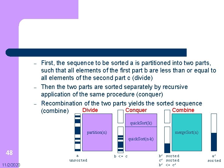
l Quicksort is one of the fastest and simplest sorting algorithms. It works recursively by a divide-and-conquer strategy: – – – 47 11/2/2020 1) Divide the problem is decomposed into subproblems 2) Conquer the subproblems are solved 3) Combine the solutions of the subproblems are recombined to the solution of the original problem

– – – First, the sequence to be sorted a is partitioned into two parts, such that all elements of the first part b are less than or equal to all elements of the second part c (divide) Then the two parts are sorted separately by recursive application of the same procedure (conquer) Recombination of the two parts yields the sorted sequence Divide Conquer Combine (combine) quick. Sort(k) partition(n) merge. Sort(n) quick. Sort(n-k) 48 11/2/2020 a unsorted b <= c b’ sorted c’ sorted b’ <= c’ a’ sorted

void quick. Sort(int[] a, int left, int right){ int temp; if (left < right){ int pivot = a[(left + right) / 2]; int i = left, j = right; while (i < j){ while (a[i] < pivot){ i++; //a[i] is "large" } while (a[j] > pivot){ j--; //a[j] is "small" } if (i <= j){ //exchange a[i] and a[j] temp = a[i]; a[i] = a[j]; a[j] = temp; i++; j--; } } // Recursively sort the "small" and //"large" subarrays of a independently quick. Sort(a, left, j); quick. Sort(a, i, right); } } 49 11/2/2020 //sort a[left. . j] //sort a[i. . right]

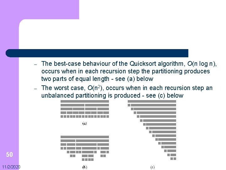
– – 50 11/2/2020 The best-case behaviour of the Quicksort algorithm, O(n log n), occurs when in each recursion step the partitioning produces two parts of equal length - see (a) below The worst case, O(n 2), occurs when in each recursion step an unbalanced partitioning is produced - see (c) below