10 Plotting Continuous Functions Linspace Array Operations Insight

10. Plotting Continuous Functions Linspace Array Operations Insight Through Computing

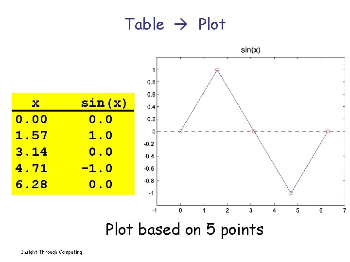
Table Plot x 0. 00 1. 57 3. 14 4. 71 6. 28 sin(x) 0. 0 1. 0 0. 0 -1. 0 0. 0 Plot based on 5 points Insight Through Computing

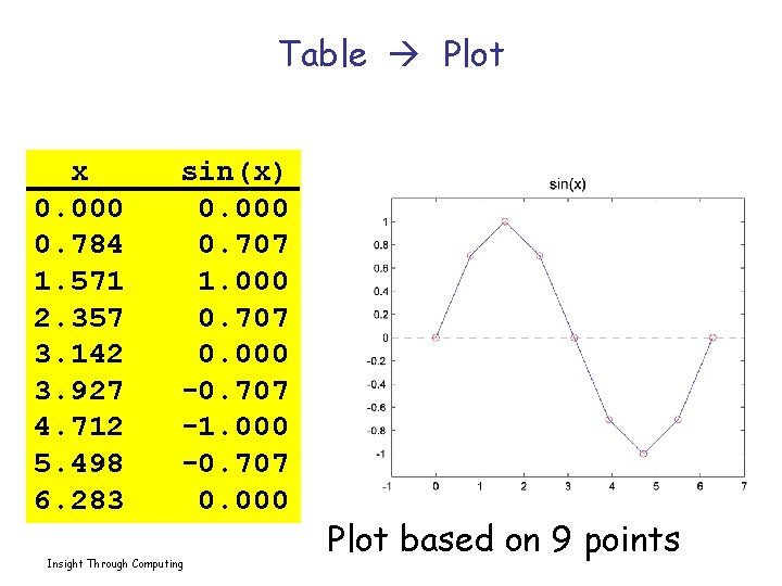
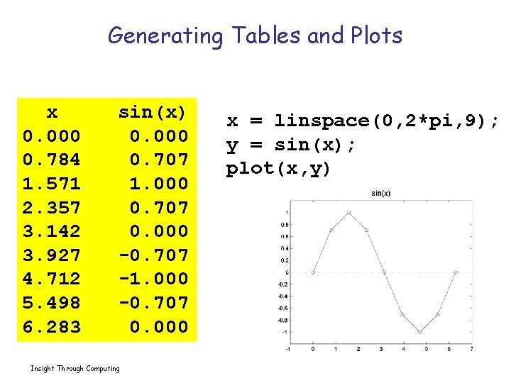
Table Plot x 0. 000 0. 784 1. 571 2. 357 3. 142 3. 927 4. 712 5. 498 6. 283 sin(x) 0. 000 0. 707 1. 000 0. 707 0. 000 -0. 707 -1. 000 -0. 707 0. 000 Insight Through Computing Plot based on 9 points

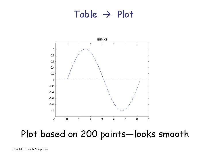
Table Plot based on 200 points—looks smooth Insight Through Computing

Generating Tables and Plots x 0. 000 0. 784 1. 571 2. 357 3. 142 3. 927 4. 712 5. 498 6. 283 sin(x) 0. 000 0. 707 1. 000 0. 707 0. 000 -0. 707 -1. 000 -0. 707 0. 000 Insight Through Computing x = linspace(0, 2*pi, 9); y = sin(x); plot(x, y)

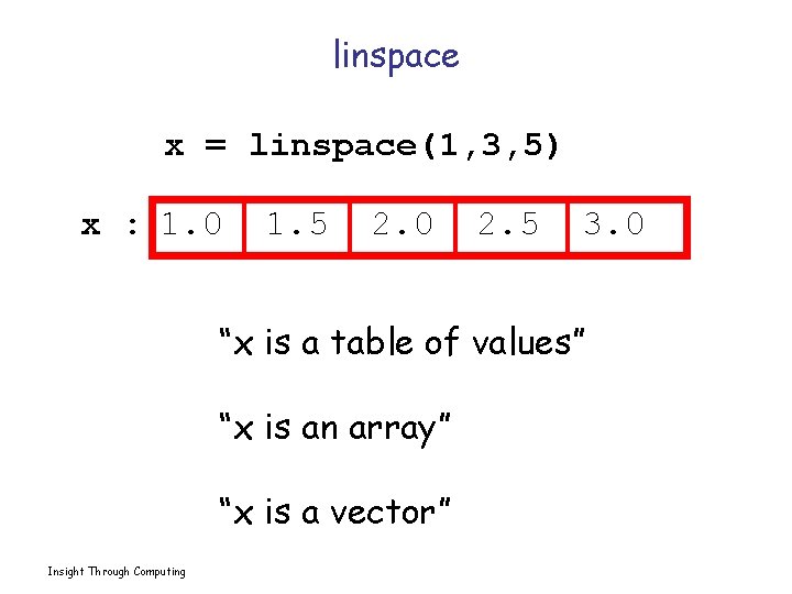
linspace x = linspace(1, 3, 5) x : 1. 0 1. 5 2. 0 2. 5 3. 0 “x is a table of values” “x is an array” “x is a vector” Insight Through Computing

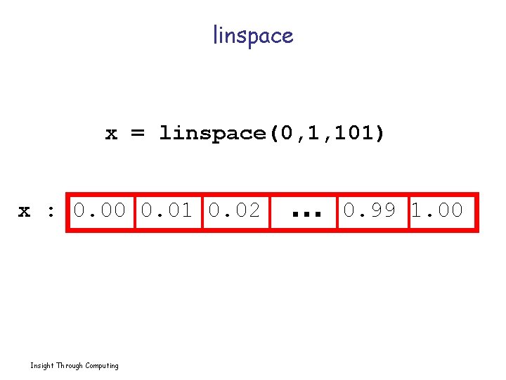
linspace x = linspace(0, 1, 101) x : 0. 00 0. 01 0. 02 Insight Through Computing … 0. 99 1. 00

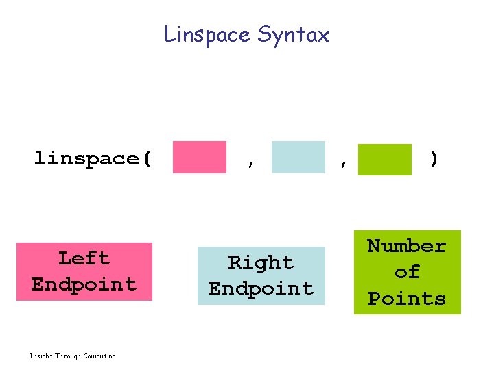
Linspace Syntax linspace( Left Endpoint Insight Through Computing , Right Endpoint , ) Number of Points

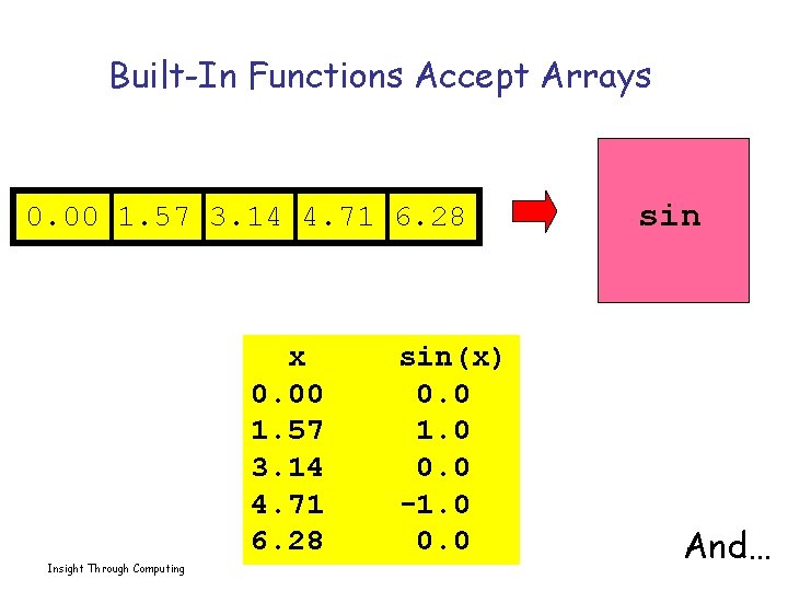
Built-In Functions Accept Arrays 0. 00 1. 57 3. 14 4. 71 6. 28 x 0. 00 1. 57 3. 14 4. 71 6. 28 Insight Through Computing sin(x) 0. 0 1. 0 0. 0 -1. 0 0. 0 sin And…

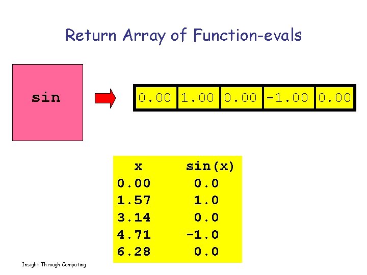
Return Array of Function-evals sin 0. 00 1. 00 0. 00 -1. 00 0. 00 x 0. 00 1. 57 3. 14 4. 71 6. 28 Insight Through Computing sin(x) 0. 0 1. 0 0. 0 -1. 0 0. 0

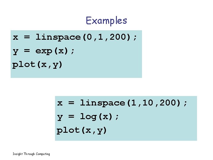
Examples x = linspace(0, 1, 200); y = exp(x); plot(x, y) x = linspace(1, 10, 200); y = log(x); plot(x, y) Insight Through Computing

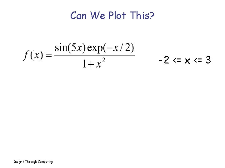
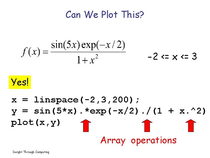
Can We Plot This? -2 <= x <= 3 Insight Through Computing

Can We Plot This? -2 <= x <= 3 Yes! x = linspace(-2, 3, 200); y = sin(5*x). *exp(-x/2). /(1 + x. ^2) plot(x, y) Array operations Insight Through Computing

Must Learn How to Operate on Arrays Look at four simpler plotting challenges. Insight Through Computing

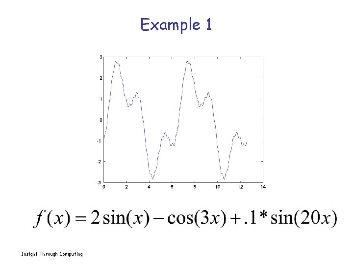
Example 1 Insight Through Computing

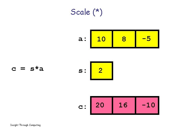
Scale (*) c = s*a Insight Through Computing a: 10 s: 2 c: 20 8 -5 16 -10

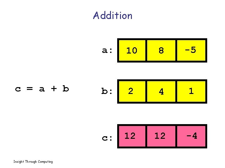
Addition c = a + b Insight Through Computing a: 10 8 -5 b: 2 4 1 c: 12 12 -4

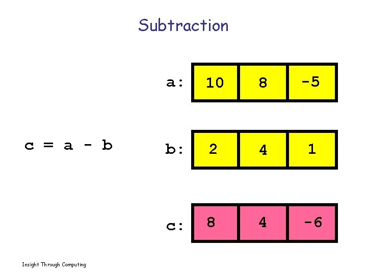
Subtraction c = a - b Insight Through Computing a: 10 8 -5 b: 2 4 1 c: 8 4 -6

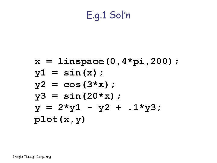
E. g. 1 Sol’n x = linspace(0, 4*pi, 200); y 1 = sin(x); y 2 = cos(3*x); y 3 = sin(20*x); y = 2*y 1 - y 2 +. 1*y 3; plot(x, y) Insight Through Computing

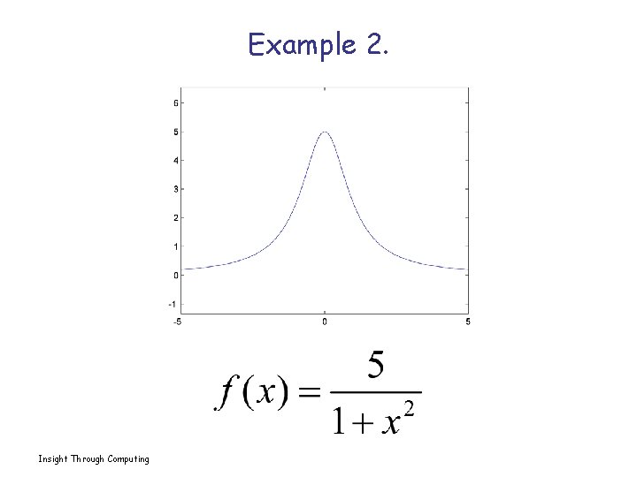
Example 2. Insight Through Computing

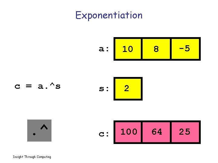
Exponentiation a: 10 c = a. ^s s: 2 . ^ c: 100 Insight Through Computing 8 -5 64 25

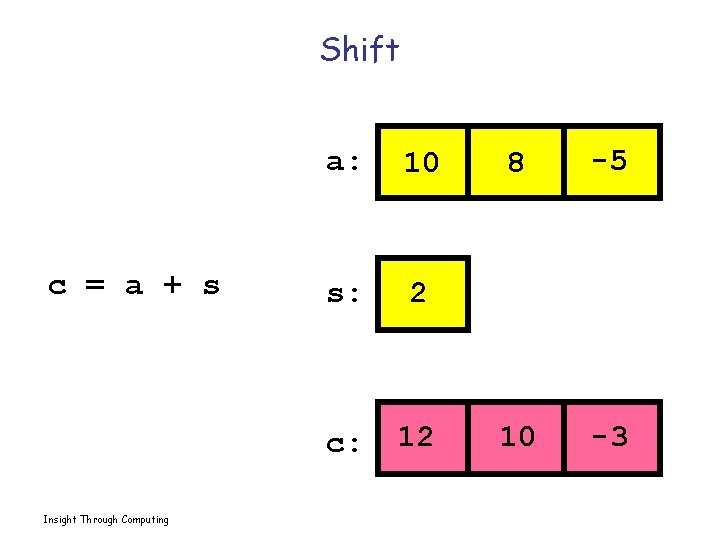
Shift c = a + s Insight Through Computing a: 10 s: 2 c: 12 8 -5 10 -3

Reciprocation a: 10 8 -5 c: . 125 -. 2 c = 1. /a Insight Through Computing

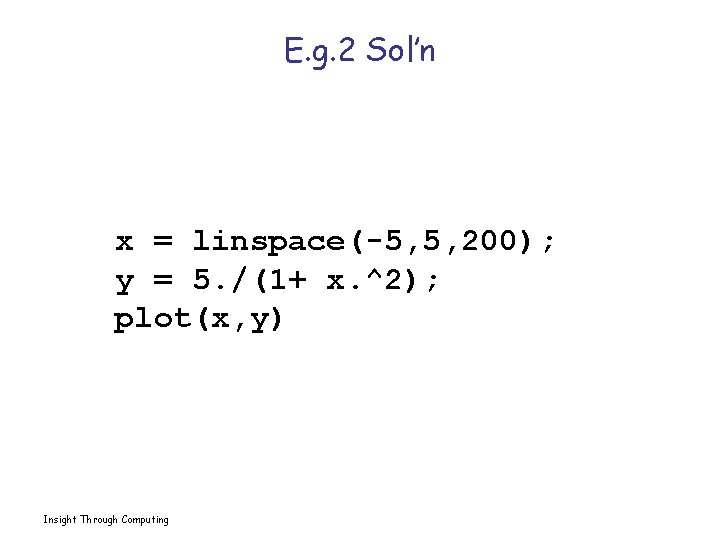
E. g. 2 Sol’n x = linspace(-5, 5, 200); y = 5. /(1+ x. ^2); plot(x, y) Insight Through Computing

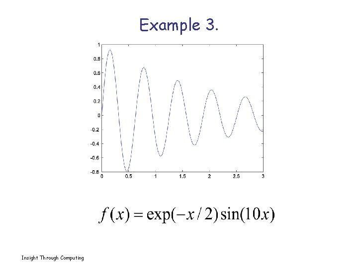
Example 3. Insight Through Computing

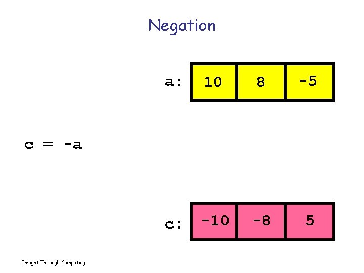
Negation a: 10 8 -5 c: -10 -8 5 c = -a Insight Through Computing

Scale (/) c = a/s Insight Through Computing a: 10 s: 2 c: 5 8 -5 4 -2. 5

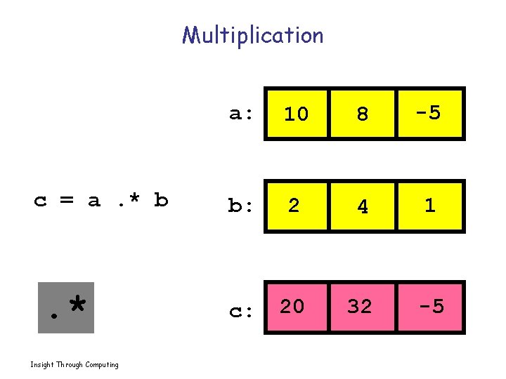
Multiplication c = a. * b . * Insight Through Computing a: 10 8 -5 b: 2 4 1 c: 20 32 -5

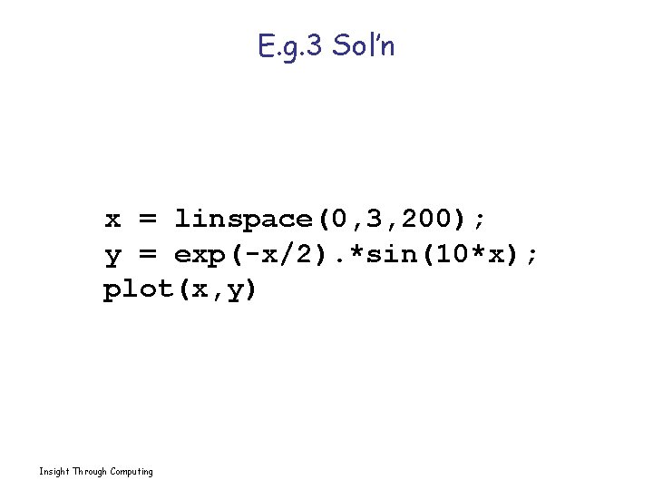
E. g. 3 Sol’n x = linspace(0, 3, 200); y = exp(-x/2). *sin(10*x); plot(x, y) Insight Through Computing

Example 4. Insight Through Computing

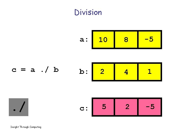
Division a: 10 8 -5 c = a. / b b: 2 4 1 . / c: 5 2 -5 Insight Through Computing

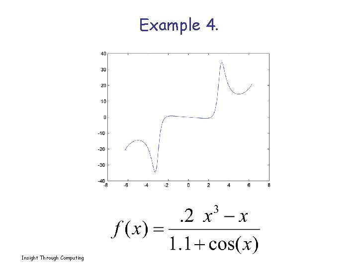
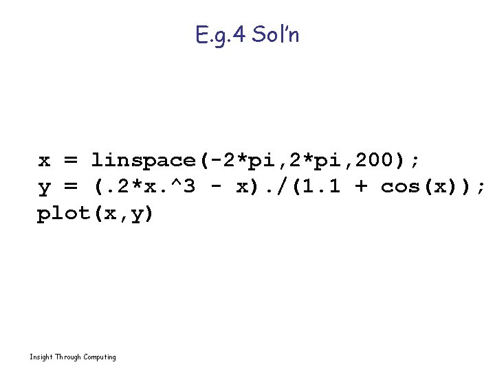
E. g. 4 Sol’n x = linspace(-2*pi, 200); y = (. 2*x. ^3 - x). /(1. 1 + cos(x)); plot(x, y) Insight Through Computing

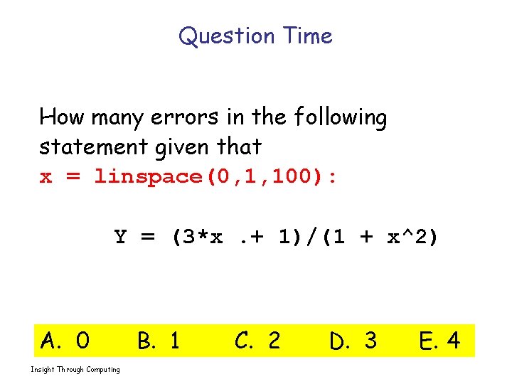
Question Time How many errors in the following statement given that x = linspace(0, 1, 100): Y = (3*x. + 1)/(1 + x^2) A. 0 Insight Through Computing B. 1 C. 2 D. 3 E. 4

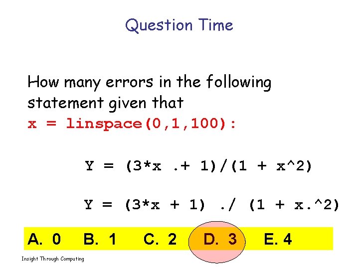
Question Time How many errors in the following statement given that x = linspace(0, 1, 100): Y = (3*x. + 1)/(1 + x^2) Y = (3*x + 1). / (1 + x. ^2) A. 0 B. 1 Insight Through Computing C. 2 D. 3 E. 4

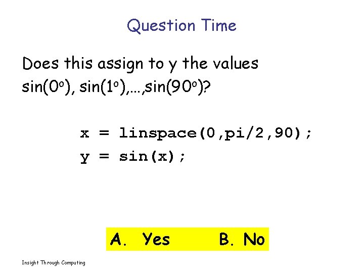
Question Time Does this assign to y the values sin(0 o), sin(1 o), …, sin(90 o)? x = linspace(0, pi/2, 90); y = sin(x); A. Yes Insight Through Computing B. No

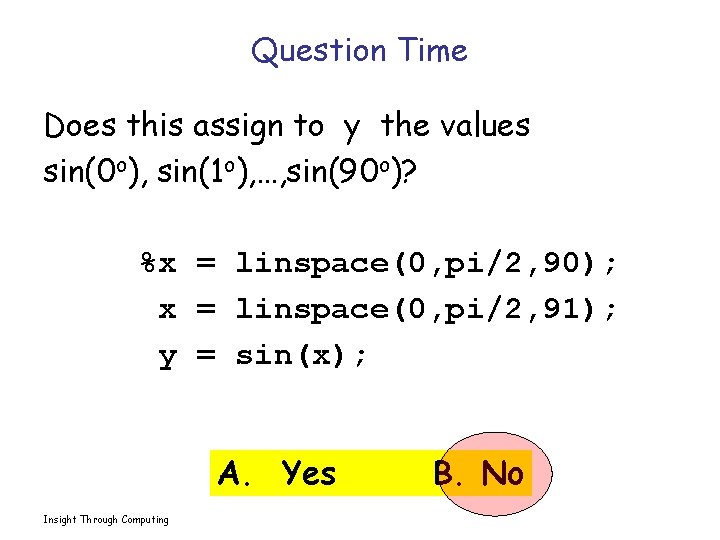
Question Time Does this assign to y the values sin(0 o), sin(1 o), …, sin(90 o)? %x = linspace(0, pi/2, 90); x = linspace(0, pi/2, 91); y = sin(x); A. Yes Insight Through Computing B. No

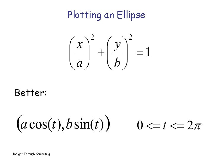
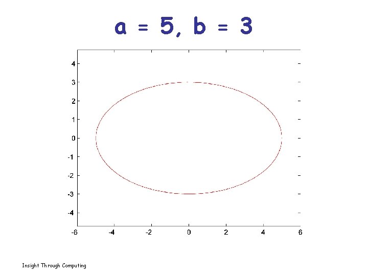
Plotting an Ellipse Better: Insight Through Computing

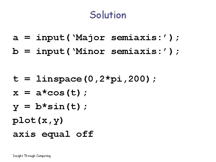
Solution a = input(‘Major semiaxis: ’); b = input(‘Minor semiaxis: ’); t = linspace(0, 2*pi, 200); x = a*cos(t); y = b*sin(t); plot(x, y) axis equal off Insight Through Computing

a = 5, b = 3 Insight Through Computing