10 D Prime Factor Algorithm 317 Ref A

10 -D Prime Factor Algorithm 317 [Ref] A. V. Oppenheim, Discrete-Time Signal Processing, London: Prentice. Hall, 3 rd ed. , 2010. N 可以是任意整數 If P 1, P 2, …, PM are small integers and prime to each other the powers k 1, k 2, …, k. M are small then using the prime factor FFT to implement the N-point DFT may require fewer real multiplications.

3 -point DFT butterfly: x[0] x[1] 318 X[0] X[1] x[2] X[2] Needs 4 complex multiplications (12 real multiplications) N–point DFT butterfly: needs 3(N 1) real multiplications 然而，可以使用特殊的方法，讓 N–point DFT 的乘法量大幅減少 (即使 N 2 k) 例如 pages 290, 297

319 Detail of the implementation method of the prime factor algorithm n = 0, 1, …. , N − 1, m = 0, 1, …. , N − 1 Case 1: 假設 N = P 1 P 2 ， P 1 is prime to P 2 拆成 P 2 個 P 1 -point DFTs，和 P 1 個 P 2 -point DFTs 令 n = ((n 1 P 1 + n 2 P 2)) N m = ((m 1 P 1 + m 2 P 2)) N n 1, m 1 = 0, 1, …. , P 2 − 1, n 2, m 2 = 0, 1, …. , P 1 − 1 當 P 1, P 2 互值時，每一個 n 1, n 2 對應到唯一一個 n (( ))N : 除以 N 的餘數

例子：當 N = 15, P 1 = 3, P 2 = 5, 0 = ((0· P 1 + 0·P 2))15 10 = ((0· P 1 + 2·P 2))15 1 = ((2· P 1 + 2·P 2))15 11 = ((2· P 1 + 1·P 2))15 2 = ((4· P 1 + 1·P 2))15 12 = ((4· P 1 + 0·P 2))15 3 = ((1· P 1 + 0·P 2))15 13 = ((1· P 1 + 2·P 2))15 4 = ((3· P 1 + 2·P 2))15 14 = ((3· P 1 + 1·P 2))15 5 = ((0· P 1 + 1·P 2))15 6 = ((2· P 1 + 0·P 2))15 7 = ((4· P 1 + 2·P 2))15 8 = ((1· P 1 + 1·P 2))15 9 = ((3· P 1 + 0·P 2))15 320

321 Step 2 Step 3 n 1, m 1 = 0, 1, …. , P 2 − 1, n 2, m 2 = 0, 1, …. , P 1 − 1

Step 1 令 Step 2 固定 n 2，對 n 1 做 P 2 -point DFT n 2 有 P 1 個值，所以有 P 1 個 P 2 -point DFTs Step 3 固定 m 3，對 n 2 做 P 1 -point DFT m 3 有 P 2 個值，所以有 P 2 個 P 1 -point DFTs m 3 = 0, 1, …. , P 2 − 1, m 4 = 0, 1, …. , P 1 − 1 Step 4 其中 ((m 1 P 1))P 2 = m 3, ((m 2 P 2))P 1 = m 4, 322

n = 0, 1, …. , N − 1, m = 0, 1, …. , N − 1 Case 2: 假設 N = P 1 P 2 ， P 1 is not prime to P 2 令 n = n 1 P 1 + n 2 m = m 1 + m 2 P 2 n 1, m 1 = 0, 1, …. , P 2 − 1, n 2, m 2 = 0, 1, …. , P 1 − 1 323

324 Step 2 Step 3 Step 4 被稱為 twiddle factor，需要額外的乘法 n 1, m 1 = 0, 1, …. , P 2 − 1, n 2, m 2 = 0, 1, …. , P 1 − 1

Step 1 令 Step 2 固定 n 2，對 n 1 作 P 2 -point DFT n 2 有 P 1 個值，所以有 P 1 個 P 2 -point DFTs Step 3 Step 4 固定 m 1，對 n 2 作 P 1 -point DFT Step 5 325

10 -E FFT 的乘法量的計算 假設 N = P 1 P 2 ， P 1 is prime to P 2 P 1 -point DFT 的乘法量為 B 1， P 2 -point DFT 的乘法量為 B 2 則 N-point DFT 的乘法量為 P 2 B 1 + P 1 B 2 假設 P 1, P 2, …. , PK 彼此互質 Pk-point DFT 的乘法量為 Bk 則 N-point DFT 可分解成 (N/P 1) 個 P 1 -point DFTs (N/P 2) 個 P 2 -point DFTs : (N/PK) 個 PK-point DFTs 總乘法量為 326

例子： 16 -point DFT, 16 = 8 2 , 乘法量 = 2 4 + 8 0 + 3 4 + 2 2 = 24 16 = 4 4 乘法量 = 4 0 + 3 4 + 2 4 = 20 328

329 10 -F Goertzel Algorithm DFT: x[n] = f [N n], n = 1, 2, …. , N x[n] F[m] = y[N] y[n] 優點： Hardware 最為精簡 缺點： 運算時間較長

10 -G Chirp Z Transform 適合於計算 FT 當 sampling interval 不為 t f 1/N 時 Continuous Fourier transform: 取 t = n t, f = m f, 當 t f = 1/N, 將可以用 DFT 以及 FFT來對上式作implementation。 當 t f 1/N 的時候 採用 CZT 330

10 -H Winograd Algorithm for DFT Implementation 331 Basic idea: Except for the 1 st row and the 1 st column, the N-point DFT is equivalent to the (N− 1)-point circular convolution when N is a prime number. Example: 5 -point DFT , = exp[ j 72 ],

332 將 3 rd and 4 th rows, 3 rd and 4 th columns 作交換 變成 circular convolution 的 型態 Circular Convolution with time inverse

333

當 N 為其他的 prime numbers 時，也可以運用 permutation 和 circular 334 convolution來計算 prime-number DFTs (Step 1) Delete the 1 st row and the 1 st column. (Step 2) Perform the row and column permutations. Rows 和 columns 的順序相同 (a) 找出一個 primitive root a, 使得 ak mod N 1 when k = 1, 2, …. , N− 2, a. N− 1 mod N 1 （Primitive root 的概念，會在後面講到數論時複習） (b) Rows 和 columns 的順序，以 p[n] 來表示， p[n] = an mod N, n = 0, 1, …. , N− 2 (Step 3) 變成 circular convolution 的型態 則 N-point DFT 可以用(N− 1)-point DFTs 來 implementation

重要理論： 335 Any N-point DFT can be implemented by the 2 k-point DFTs whatever the value of N is. 7 -point DFT 123 -point DFT

XI. Discrete Fourier Transform 的替代方案 11 -A Why Should We Use Other Operations? Discrete Fourier Transform (DFT): 優點： 有 fast algorithm (complexity 為 O(Nlog 2 N)). 適合做頻譜分析和 convolution implementation 問題： (1) complex output (2) The exponential function is not of the binary form. 336

337 Applications of the DFT: Spectrum analysis Performing the convolution For spectrum analysis, the DFT can be replaced by: (1) DCT, (2) DST, (3) DHT, (4) Walsh (Hadamard) transform, (5) Haar transform, (6) orthogonal basis expansion, (including orthogonal polynomials and CDMA), (7) wavelet transform, (8) time-frequency distribution When performing the convolution, the DFT can be replaced by: (1) DCT, (2) DST, (3) DHT, (4) Directly Computing, (5) Sectioned DFT convolution, (6) Winograd algorithm, (7) Walsh (Hadamard) transform, (8) number theoretic transform (NTT)

11 -B Discrete Sinusoid Transforms DCT (discrete cosine transform) has 8 types DST (discrete sine transform) has 8 types DHT (discrete Hartley transform) has 4 types 共通的特性：皆為 real, 且和 DFT 密切相關 Reference N. Ahmed, T. Natarajan, and K. R. Rao, “Discrete cosine transform, ” IEEE Trans. Comput. , vol. C-23, pp. 90 -93, Jan 1974. Z. Cvetkovic and M. V. Popovic, “New fast recursive algorithms for the computation of discrete cosine and sine transforms, ” IEEE Trans. Signal Processing, vol. 40, pp. 2083 -2086, Aug. 1992. R. N. Bracewell, The Hartley Transform, New York, Oxford University Press, 1986. S. C. Chan and K. L. Ho, “Prime factor real-valued Fourier, cosine and Hartley transform, ” Proc. Signal Processing VI, pp. 1045 -1048, 1992. 338

340 (Proof) When x[n] = x[N−n] ，N is even (The case where N is odd can be proved in the similar way)

341 half part of x[n] 25

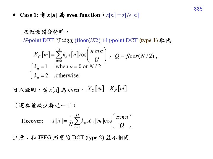
Case 3: 當 x[n] 為 real function，在做頻譜分析時， N-point DFT 可以被 N-point DHT (type 1) 取代 , where cas(k) = cos(k) + sin(k) 比較： exp(jk) = cos(k) + jsin(k) 可以證明，若 x[n] 為 real， (運算量減少將近一半) Recover: 343

大部分的 convolution 仍然使用 DFT。 y[n] = x[n] h[n] y[n] = IDFT{ DFT(x[n]) {DFT(h[n]) } 思考：何時適合用 DCT 做 convolution ？ 何時適合用 DST 做 convolution ？ 何時適合用 DHT 做 convolution ？ 344

349 (12) Reference 的寫法 (以 IEEE Transactions on Signal Processing 為例) (A) Journal papers and conference papers Authors (first name 或 middle name 只用一個字母代表), “title , ” name of the journal (縮寫為佳), vol. *, no. *, pp. **~**, month, year. 使用縮寫 逗號在引號之前 只有第一個字母、專有名詞 加句號 開頭、和縮為用大寫 範例： S. Abe and J. T. Sheridan, “Optical operations on wave functions as the Abelian subgroups of the special affine Fourier transformation, ” Opt. Lett. , vol. 19, no. 22, pp. 1801 -1803, 1994.

(B) Books 350 Authors (first name 或 middle name 只用一個字母代表), title (斜體, 字開頭 大寫，不加引號), 第幾版 (非必需), 出版社, 出版地, year. 範例 H. M. Ozaktas, Z. Zalevsky, and M. A. Kutay, The Fractional Fourier Transform with Applications in Optics and Signal Processing, 1 st Ed. , John Wiley & Sons, New York, 2000. (C) Websites Authors, “title, ” available in http: //網址. 範例 張智星, “Utility toolbox, ” available in http: //neural. cs. nthu. edu. tw/jang/ matlab/toolbox/utility/.