10 Basic Regressions with Times Series Data 10

10. Basic Regressions with Times Series Data 10. 1 The Nature of Time Series Data 10. 2 Examples of Time Series Regression Models 10. 3 Finite Sample Properties of OLS Under Classical Assumptions 10. 4 Functional Form, Dummy Variables, and Index Numbers 10. 5 Trends and Seasonality

10. 1 Nature of Time Series Time series data is any data that follows one observation (location, person, etc) over time -temporal ordering is very important for time series data (higher observations correspond to more recent data) -this is due to the fact that the past can affect the future but not the other way around -recall that for cross-sectional data ordering was of little importance -a sequence of random variables indexed by time is call a STOCHASTIC (random) PROCESS or TIME SERIES PROCESS

10. 1 Random Time Series How is time series data considered to be random? 1) We don’t know the future. 2) There a variety of variables that impact the future. 3) Future outcomes are thus random variables. -Each data point is one possible outcome, or realization -If certain conditions were different, the realization could have been different -but we don’t have a time machine to go back in time and obtain this realization

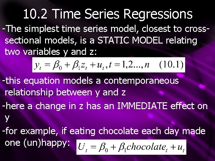
10. 2 Time Series Regressions -The simplest time series model, closest to crosssectional models, is a STATIC MODEL relating two variables y and z: -this equation models a contemporaneous relationship between y and z -here a change in z has an IMMEDIATE effect on y -for example, if eating chocolate each day made one (un)happy:

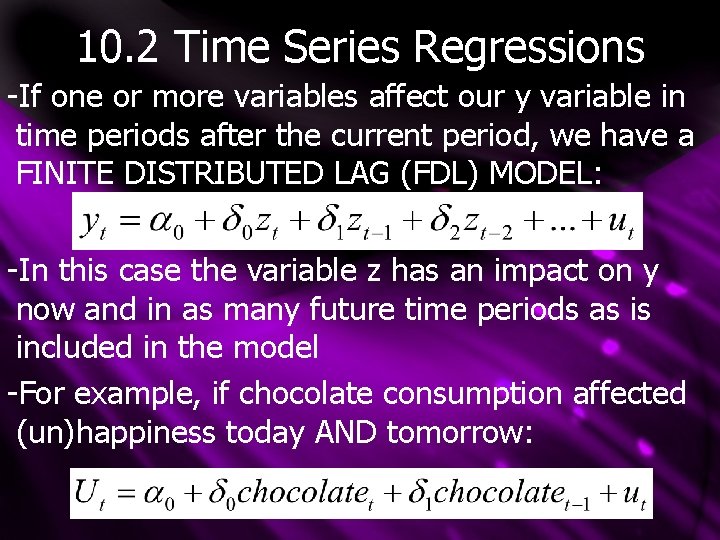
10. 2 Time Series Regressions -If one or more variables affect our y variable in time periods after the current period, we have a FINITE DISTRIBUTED LAG (FDL) MODEL: -In this case the variable z has an impact on y now and in as many future time periods as is included in the model -For example, if chocolate consumption affected (un)happiness today AND tomorrow:

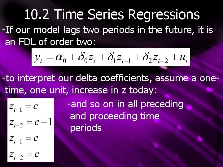
10. 2 Time Series Regressions -If our model lags two periods in the future, it is an FDL of order two: -to interpret our delta coefficients, assume a onetime, one unit, increase in z today: -and so on in all preceding and proceeding time periods

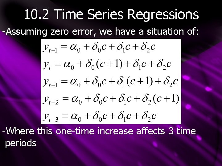
10. 2 Time Series Regressions -Assuming zero error, we have a situation of: -Where this one-time increase affects 3 time periods

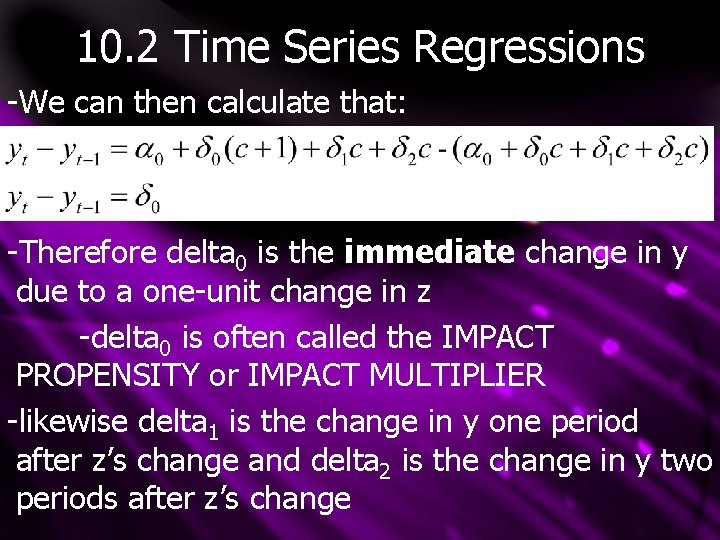
10. 2 Time Series Regressions -We can then calculate that: -Therefore delta 0 is the immediate change in y due to a one-unit change in z -delta 0 is often called the IMPACT PROPENSITY or IMPACT MULTIPLIER -likewise delta 1 is the change in y one period after z’s change and delta 2 is the change in y two periods after z’s change

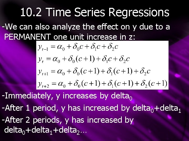
10. 2 Time Series Regressions -We can also analyze the effect on y due to a PERMANENT one unit increase in z: -Immediately, y increases by delta 0 -After 1 period, y has increased by delta 0+delta 1 -After 2 periods, y has increased by delta 0+delta 1+delta 2…

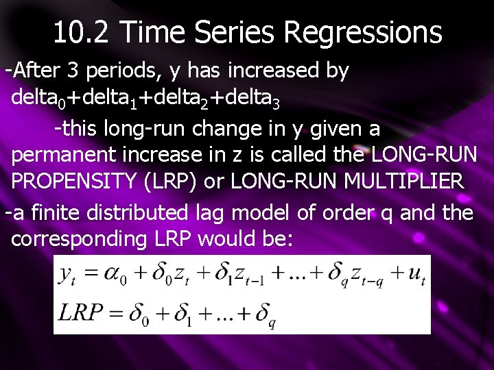
10. 2 Time Series Regressions -After 3 periods, y has increased by delta 0+delta 1+delta 2+delta 3 -this long-run change in y given a permanent increase in z is called the LONG-RUN PROPENSITY (LRP) or LONG-RUN MULTIPLIER -a finite distributed lag model of order q and the corresponding LRP would be:

10. 2 Time Series Regressions -Note that the long-run propensity (LRP) of a time series regression cause high multicollinearity -Therefore it is often not possible to obtain precise estimates of each delta, but rather we obtain a good estimate of the LRP. -note that different sources use either t=0 or t=1 as the base year -our text considers t=1 the base year

10. 3 Finite Sample Properties of OLS under Classical Assumptions -in this section we will see how the 6 Classical Linear model (CLM) assumptions are modified from their time-series form in order to imply to finite (small) sample properties of OLS in time series regressions Note that xtj refers to the t’th time period, where j is labels the x variable Xt will refer to all x observations at time t X will refer to a matrix including all x observations over all times t

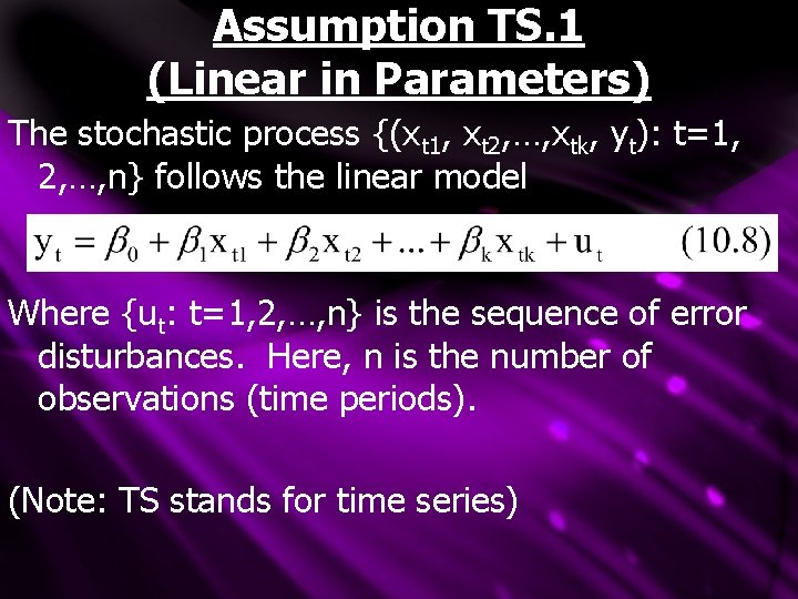
Assumption TS. 1 (Linear in Parameters) The stochastic process {(xt 1, xt 2, …, xtk, yt): t=1, 2, …, n} follows the linear model Where {ut: t=1, 2, …, n} is the sequence of error disturbances. Here, n is the number of observations (time periods). (Note: TS stands for time series)

Assumption TS. 2 (No Perfect Collinearity) In the sample (and therefore in the underlying time series process), no independent variable is constant nor a perfect linear combination of the others

10. 3 Assumption Notes -Our first two assumptions are almost identical to their cross-sectional counterparts -Note that TS. 2 allows for correlation between variables, it only disallows PERFECT correlation -the final assumption for time series OLS unbiasedness replaces MLR. 4 and obviates the need for a random sampling assumption:

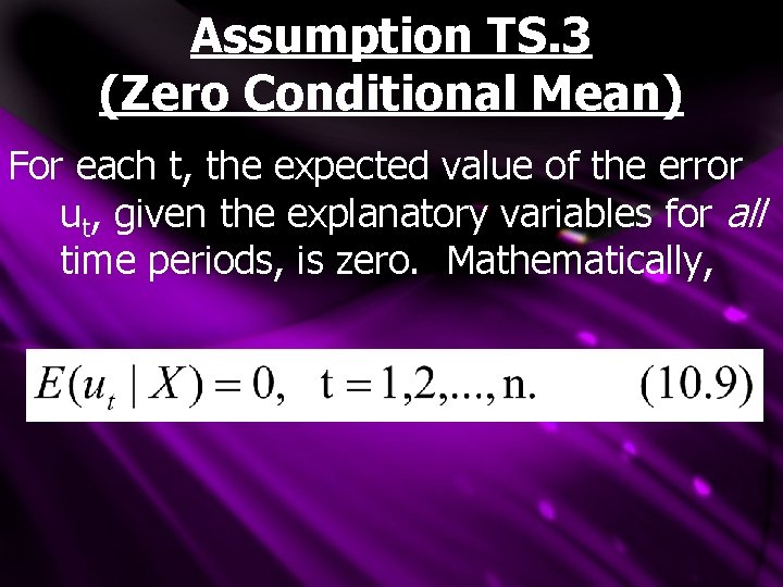
Assumption TS. 3 (Zero Conditional Mean) For each t, the expected value of the error ut, given the explanatory variables for all time periods, is zero. Mathematically,

10. 3 Assumption TS. 3 Notes -TS. 3 assumes that our error term (unaccounted for variables) is uncorrelated with our included variables IN EVERY TIME PERIOD -this requires us to correctly specify the functional form (static or lag) between y and z -if ut is independent of X and E(ut)=0, TS. 3 automatically holds -such a strong assumption was not needed in cross sectional data because each observation was random; in time series each observation is sequential

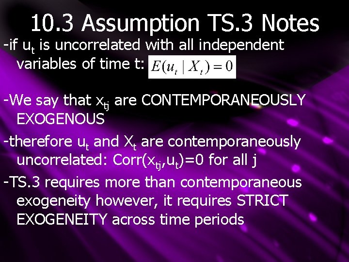
10. 3 Assumption TS. 3 Notes -if ut is uncorrelated with all independent variables of time t: -We say that xtj are CONTEMPORANEOUSLY EXOGENOUS -therefore ut and Xt are contemporaneously uncorrelated: Corr(xtj, ut)=0 for all j -TS. 3 requires more than contemporaneous exogeneity however, it requires STRICT EXOGENEITY across time periods

10. 3 Assumption TS. 3 Notes -Note that TS. 3 puts no restrictions on correlation between independent variables across time -Note that TS. 3 puts no restrictions on correlation between error terms across time TS. 3 can fail due to: 1) Omitted variables 2) Measurement error 3) Misspecified Model 4) Other

10. 3 TS. 3 Failure -If a variable z has a LAGGED effect on y, its lag must be included in the model or TS. 3 is violated -never use a static model if a lag model is more appropriate -ie: overeating (z) last month (ie: Christmas) causes more exercise in this month (y) -TS. 3 also fails if ut affects future zt (since only past zt are controlled for) -ie: cold weather last month (u) will cause depression thus under eating next month (z)

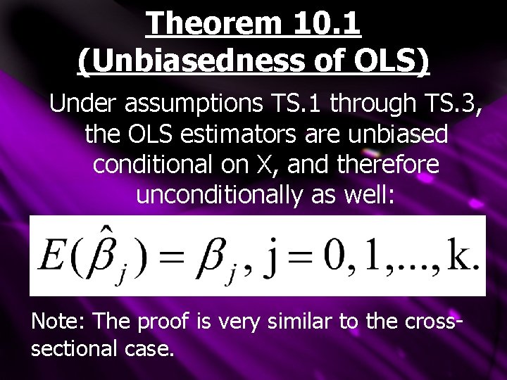
Theorem 10. 1 (Unbiasedness of OLS) Under assumptions TS. 1 through TS. 3, the OLS estimators are unbiased conditional on X, and therefore unconditionally as well: Note: The proof is very similar to the crosssectional case.