10 3 Regression College Prep Stats Objectives 1
10 -3 Regression College Prep Stats
Objectives 1) The basic concepts related to regression. 2) Finding the equation of the straight line that best fits the paired sample data. 3) Using the regression equation for predictions. 4) Graphing and interpreting the regression equation.
Learning Outcomes After this lesson, student will be able to v master the basic concepts of regression; v find out the regression equation from calculator based on the given data set; v graph the regression equation; v predict the response variable value at the given predictor variable value. v interpret the regression equation.
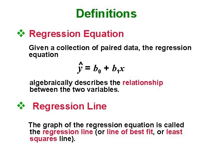
Definitions v Regression Equation Given a collection of paired data, the regression equation y^ = b 0 + b 1 x algebraically describes the relationship between the two variables. v Regression Line The graph of the regression equation is called the regression line (or line of best fit, or least squares line).
Example
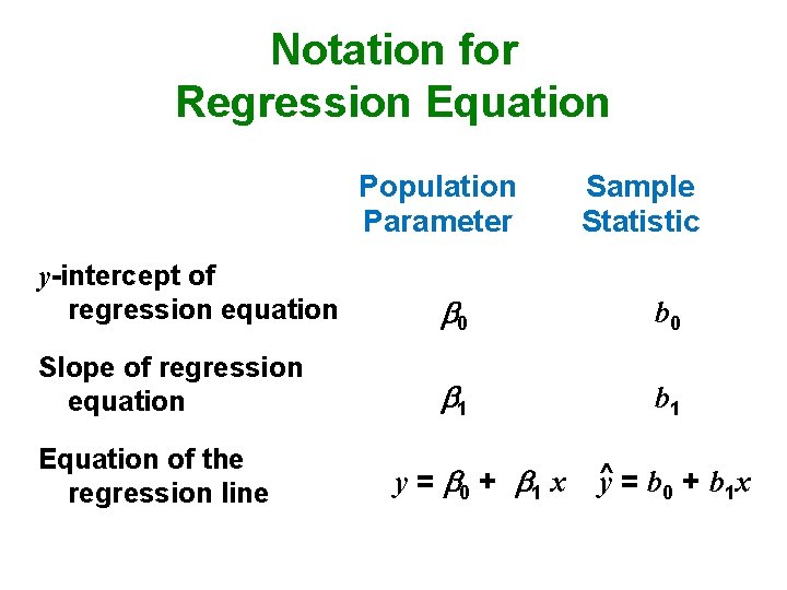
Notation for Regression Equation Population Parameter Sample Statistic y-intercept of regression equation 0 b 0 Slope of regression equation 1 b 1 Equation of the regression line y = 0 + 1 x ^ y = b 0 + b 1 x
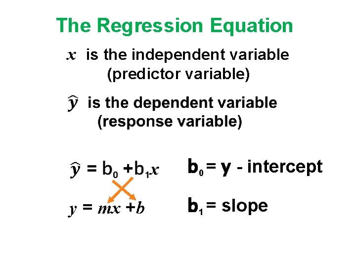
The Regression Equation x is the independent variable (predictor variable) b 0 = y - intercept y = mx +b b 1 = slope
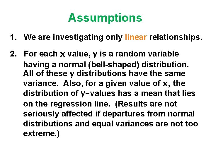
Assumptions 1. We are investigating only linear relationships. 2. For each x value, y is a random variable having a normal (bell-shaped) distribution. All of these y distributions have the same variance. Also, for a given value of x, the distribution of y-values has a mean that lies on the regression line. (Results are not seriously affected if departures from normal distributions and equal variances are not too extreme. )
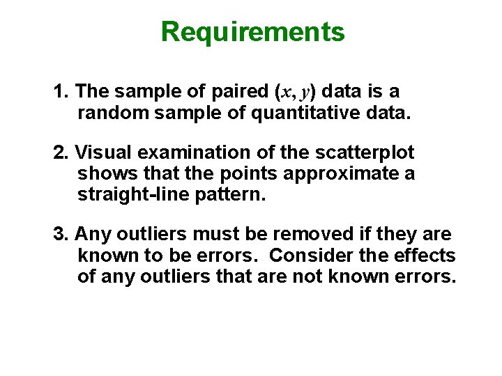
Requirements 1. The sample of paired (x, y) data is a random sample of quantitative data. 2. Visual examination of the scatterplot shows that the points approximate a straight-line pattern. 3. Any outliers must be removed if they are known to be errors. Consider the effects of any outliers that are not known errors.
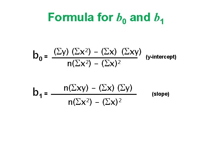
Formula for b 0 and b 1 b 0 = ( y) ( x 2) - ( x) ( xy) n( x 2) - ( x)2 b 1 = n( xy) - ( x) ( y) n( x 2) - ( x)2 (y-intercept) (slope)
Special Property The regression line fits the sample points best.
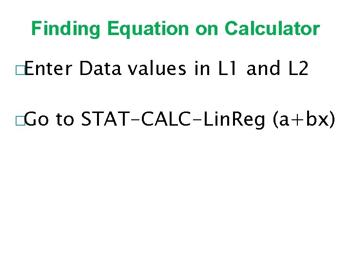
Finding Equation on Calculator �Enter �Go Data values in L 1 and L 2 to STAT-CALC-Lin. Reg (a+bx)
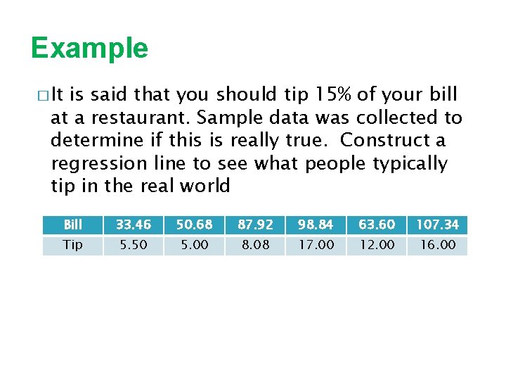
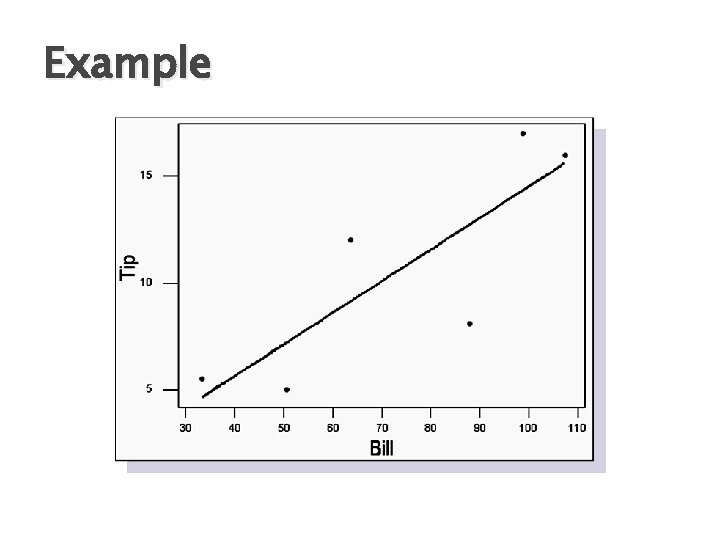
Example � It is said that you should tip 15% of your bill at a restaurant. Sample data was collected to determine if this is really true. Construct a regression line to see what people typically tip in the real world Bill 33. 46 50. 68 87. 92 98. 84 63. 60 107. 34 Tip 5. 50 5. 00 8. 08 17. 00 12. 00 16. 00
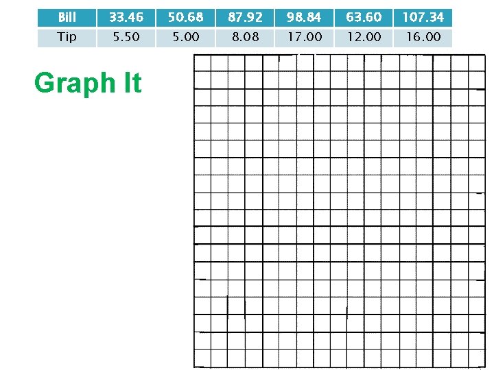
Bill 33. 46 50. 68 87. 92 98. 84 63. 60 107. 34 Tip 5. 50 5. 00 8. 08 17. 00 12. 00 16. 00 Graph It
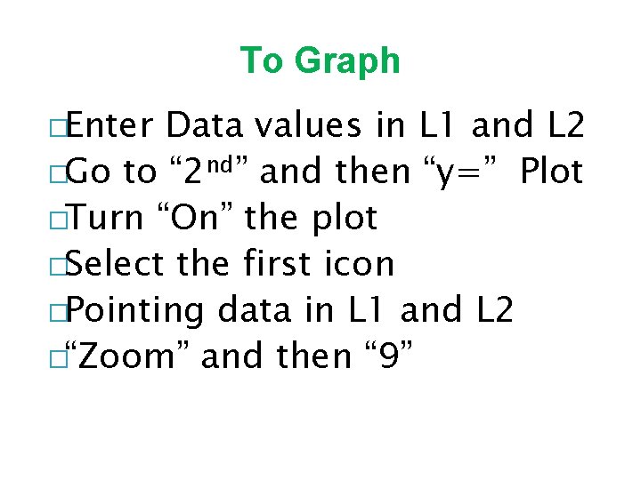
To Graph �Enter Data values in L 1 and L 2 �Go to “ 2 nd” and then “y=” Plot �Turn “On” the plot �Select the first icon �Pointing data in L 1 and L 2 �“Zoom” and then “ 9”
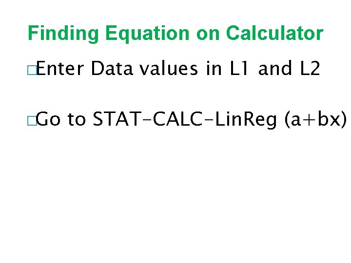
Finding Equation on Calculator �Enter �Go Data values in L 1 and L 2 to STAT-CALC-Lin. Reg (a+bx)
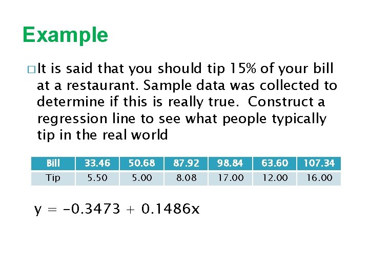
Example � It is said that you should tip 15% of your bill at a restaurant. Sample data was collected to determine if this is really true. Construct a regression line to see what people typically tip in the real world Bill 33. 46 50. 68 87. 92 98. 84 63. 60 107. 34 Tip 5. 50 5. 00 8. 08 17. 00 12. 00 16. 00 y = -0. 3473 + 0. 1486 x
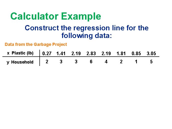
Calculator Example Construct the regression line for the following data: Data from the Garbage Project x Plastic (lb) y Household 0. 27 1. 41 2 3 2. 19 2. 83 2. 19 1. 81 0. 85 3. 05 3 6 4 2 1 5
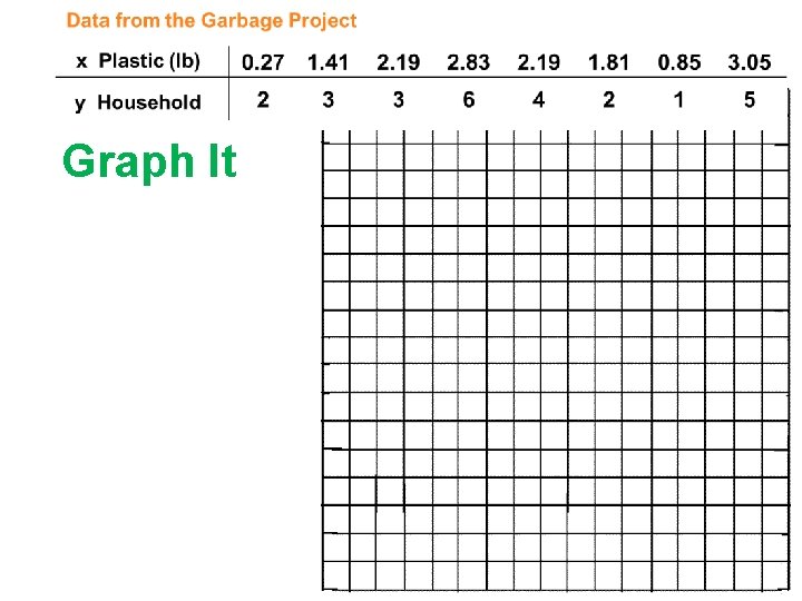
Graph It
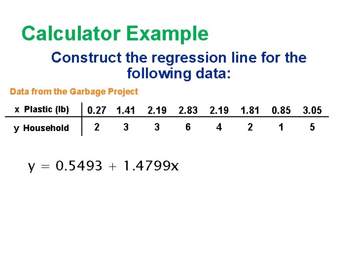
Calculator Example Construct the regression line for the following data: Data from the Garbage Project x Plastic (lb) y Household 0. 27 1. 41 2 3 2. 19 2. 83 2. 19 1. 81 0. 85 3. 05 3 6 4 2 1 5 y = 0. 5493 + 1. 4799 x
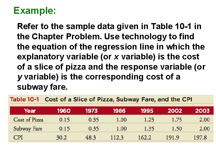
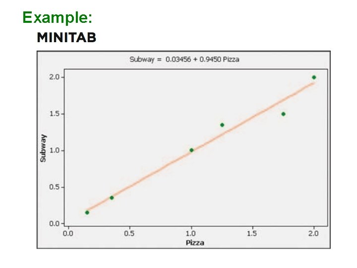
Example: Refer to the sample data given in Table 10 -1 in the Chapter Problem. Use technology to find the equation of the regression line in which the explanatory variable (or x variable) is the cost of a slice of pizza and the response variable (or y variable) is the corresponding cost of a subway fare.
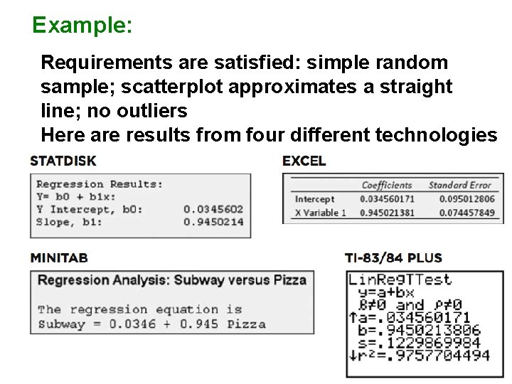
Example: Requirements are satisfied: simple random sample; scatterplot approximates a straight line; no outliers Here are results from four different technologies
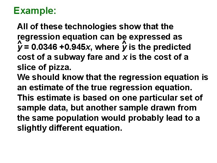
Example: All of these technologies show that the regression equation can be expressed as ^ = 0. 0346 +0. 945 x, where y ^ is the predicted y cost of a subway fare and x is the cost of a slice of pizza. We should know that the regression equation is an estimate of the true regression equation. This estimate is based on one particular set of sample data, but another sample drawn from the same population would probably lead to a slightly different equation.
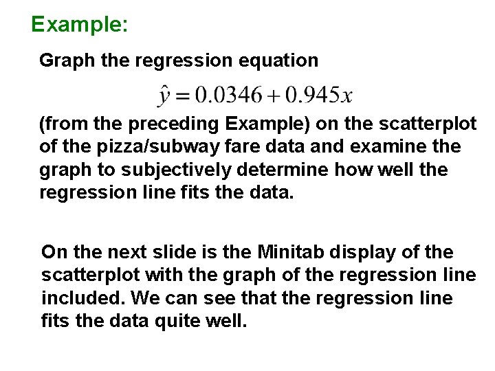
Example: Graph the regression equation (from the preceding Example) on the scatterplot of the pizza/subway fare data and examine the graph to subjectively determine how well the regression line fits the data. On the next slide is the Minitab display of the scatterplot with the graph of the regression line included. We can see that the regression line fits the data quite well.
Example:
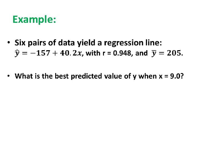
Using the Regression Equation for Predictions 1. Use the regression equation for predictions only if the graph of the regression line on the scatterplot confirms that the regression line fits the points reasonably well. 2. Use the regression equation for predictions only if the linear correlation coefficient r indicates that there is a linear correlation between the two variables (as described in Section 10 -2).
Using the Regression Equation for Predictions 3. Use the regression line for predictions only if the data do not go much beyond the scope of the available sample data. (Predicting too far beyond the scope of the available sample data is called extrapolation, and it could result in bad predictions. ) 4. If the regression equation does not appear to be useful for making predictions, the best predicted value of a variable is its point estimate, which is its sample mean.
Strategy for Predicting Values of Y
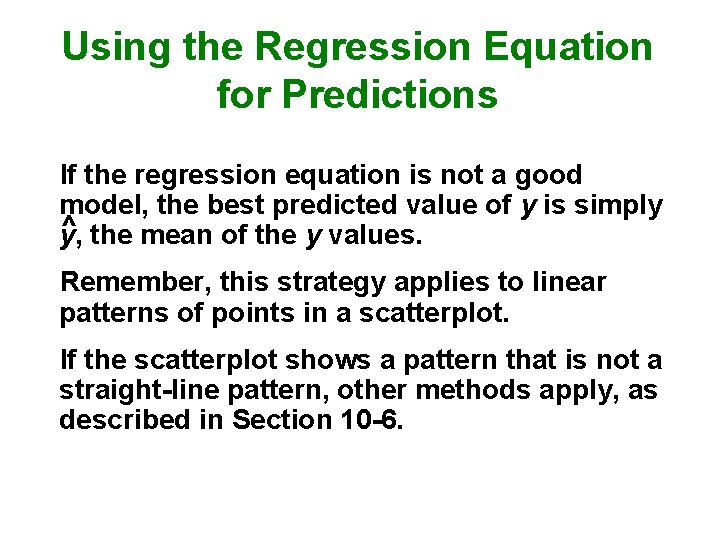
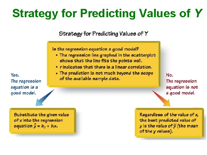
Using the Regression Equation for Predictions If the regression equation is not a good model, the best predicted value of y is simply ^ the mean of the y values. y, Remember, this strategy applies to linear patterns of points in a scatterplot. If the scatterplot shows a pattern that is not a straight-line pattern, other methods apply, as described in Section 10 -6.
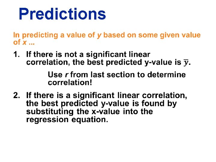
Predictions
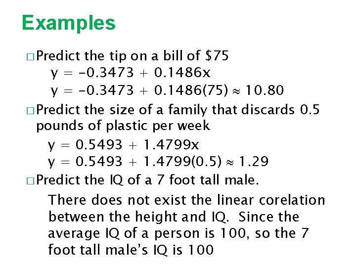
Examples � Predict the tip on a bill of $75 y = -0. 3473 + 0. 1486 x y = -0. 3473 + 0. 1486(75) 10. 80 � Predict the size of a family that discards 0. 5 pounds of plastic per week y = 0. 5493 + 1. 4799 x y = 0. 5493 + 1. 4799(0. 5) 1. 29 � Predict the IQ of a 7 foot tall male. There does not exist the linear corelation between the height and IQ. Since the average IQ of a person is 100, so the 7 foot tall male’s IQ is 100
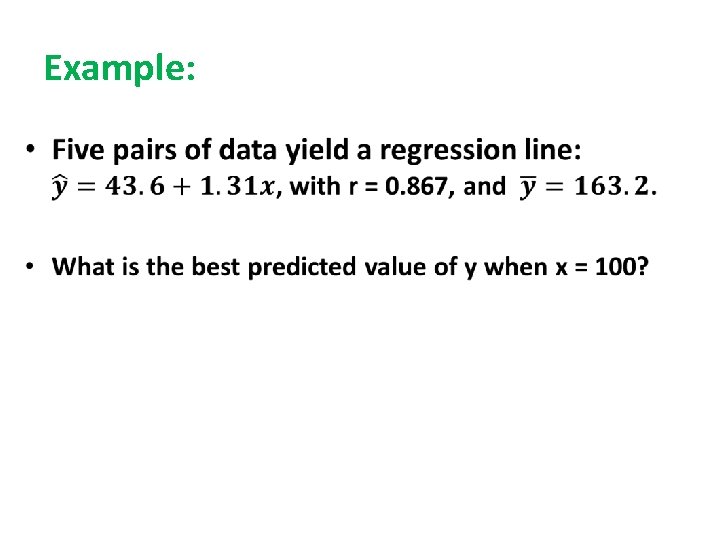
Example: •
Example: •
Recap In this section we have discussed: v The basic concepts of regression. v Using the regression equation for predictions. v Interpreting the regression equation.
Homework � P. 549: 15 -19
- Slides: 35