10 3 fminsearch n error Measure 1 m


的方法,函式 error. Measure 1 須改寫成 error. Measure 2 n 範例10")

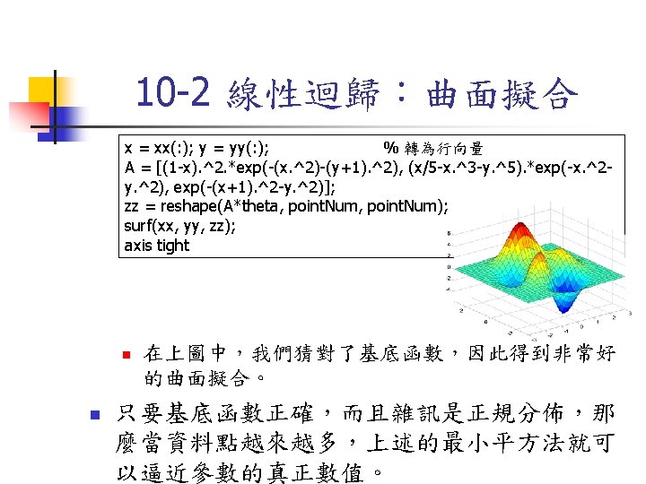
; subplot(2, 1, 1) plot(x, log(y), 'o', x, A*theta);")

- Slides: 47
10 -3 非線性迴歸:使用 fminsearch n 假設此函式為 error. Measure 1. m, n 範例10 -8: error. Measure 01. m function squared. Error = error. Measure 1(theta, data) x = data(: , 1); y = data(: , 2); y 2 = theta(1)*exp(theta(3)*x)+theta(2)*exp(theta(4)*x); squared. Error = sum((y-y 2). ^2); n 其中 theta 是參數向量,包含了 、 、λ 1 及 λ 2,data 則是觀察到的資料點,傳回的值 則是 總平方誤差。
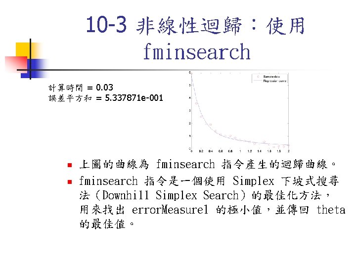
10 -3 非線性迴歸:使用 fminsearch n 欲求出 的最小值,我們可使用 fminsearch 指令 n 範例10 -9: nonlinear. Fit 01. m load data. txt theta 0 = [0 0 0 0]; tic theta = fminsearch(@error. Measure 1, theta 0, [], data); fprintf('計算時間 = %gn', toc); x = data(: , 1); y = data(: , 2); y 2 = theta(1)*exp(theta(3)*x)+theta(2)*exp(theta(4)*x); plot(x, y, 'ro', x, y 2, 'b-'); legend('Sample data', 'Regression curve'); fprintf('誤差平方和 = %dn', sum((y-y 2). ^2));
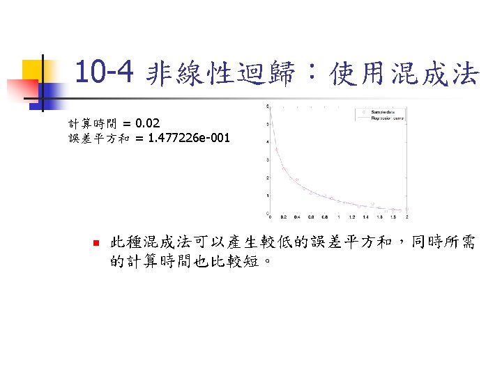
10 -4 非線性迴歸:使用混成法 n 使用上述混成(Hybrid)的方法,函式 error. Measure 1 須改寫成 error. Measure 2 n 範例10 -10: error. Measure 2. m function squared. Error = error. Measure 2(lambda, data) x = data(: , 1); y = data(: , 2); A = [exp(lambda(1)*x) exp(lambda(2)*x)]; a = Ay; y 2 = a(1)*exp(lambda(1)*x)+a(2)*exp(lambda(2)*x); squared. Error = sum((y-y 2). ^2); n lambda 是非線性參數向量, data 仍是觀察到的 資料點,a 是利用最小平方法算出的最佳線性參數 向量,傳回的 square. Error 仍是總平方誤差
10 -4 非線性迴歸:使用混成法 n 欲用此混成法求出誤差平方和的最小值 n 範例10 -11: nonlinear. Fit 02. m load data. txt lambda 0 = [0 0]; tic lambda = fminsearch(@error. Measure 2, lambda 0, [], data); fprintf('計算時間 = %gn', toc); x = data(: , 1); y = data(: , 2); A = [exp(lambda(1)*x) exp(lambda(2)*x)]; a = Ay; y 2 = a(1)*exp(lambda(1)*x)+a(2)*exp(lambda(2)*x); plot(x, y, 'ro', x, y 2, 'b-'); legend('Sample data', 'Regression curve'); fprintf('誤差平方和 = %dn', sum((y-y 2). ^2));
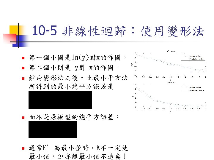
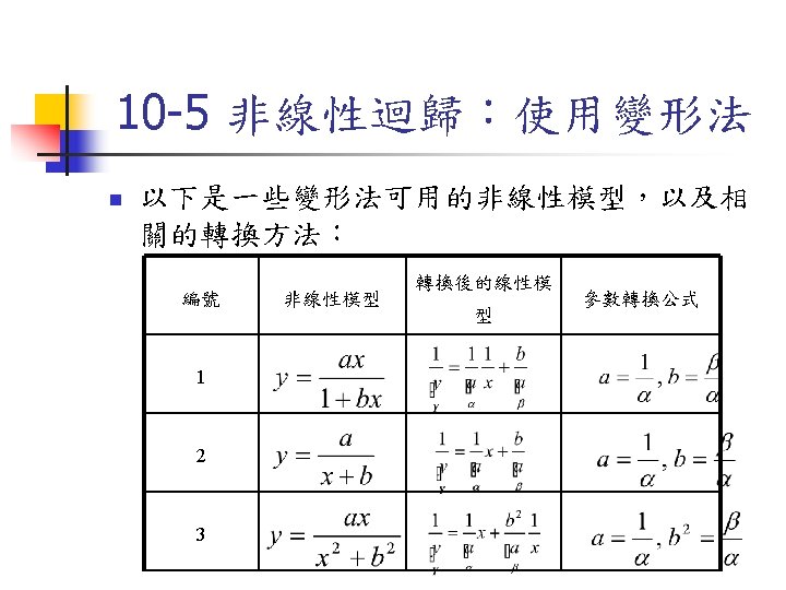
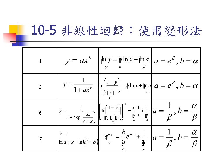
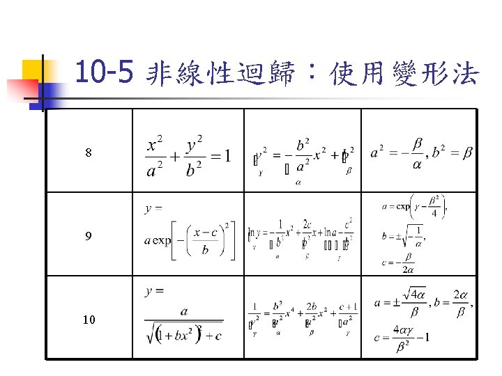
10 -5 非線性迴歸:使用變形法 theta = Alog(y); subplot(2, 1, 1) plot(x, log(y), 'o', x, A*theta); xlabel('x'); ylabel('ln(y)'); title('ln(y) vs. x'); legend('Actual value', 'Predicted value'); a = exp(theta(1)) % 辨識得到之參數 b = theta(2) % 辨識得到之參數 y 2 = a*exp(b*x); subplot(2, 1, 2); plot(x, y, 'o', x, y 2); xlabel('x'); ylabel('y'); legend('Actual value', 'Predicted value'); title('y vs. x'); fprintf('誤差平方和 = %dn', sum((y-y 2). ^2)); a = 4. 3282 b =-1. 8235 誤差平方和 = 8. 744185 e-001
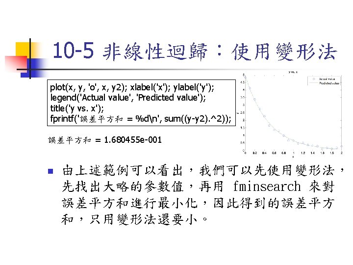
10 -5 非線性迴歸:使用變形法 n 若要求取 E的最小值,可再用 fminsearch , 並以最小平方法得到的 a 及 b 為搜尋的起點 n 範例10 -13: transform. Fit 02. m load data 2. txt x = data 2(: , 1); % 已知資料點的 x 座標 y = data 2(: , 2); % 已知資料點的 y 座標 A = [ones(size(x)) x]; theta = Alog(y); a = exp(theta(1)) % 辨識得到之參數 b = theta(2) % 辨識得到之參數 theta 0 = [a, b]; % fminsearch 的啟始參數 theta = fminsearch(@error. Measure 3, theta 0, [], data 2); x = data 2(: , 1); y = data 2(: , 2); y 2 = theta(1)*exp(theta(2)*x);