1 Time Domain Representation of Signals and Systems
![Discrete-Time Signals • In some applications, a discrete-time sequence {x[n]} may be generated by Discrete-Time Signals • In some applications, a discrete-time sequence {x[n]} may be generated by](https://slidetodoc.com/presentation_image_h2/5502f711d94db79e3c52a97e07b4827b/image-6.jpg)
![Discrete-Time Signals • Here, n-th sample is given by: x[n]= xa(t)|t=n. T= xa(n. T), Discrete-Time Signals • Here, n-th sample is given by: x[n]= xa(t)|t=n. T= xa(n. T),](https://slidetodoc.com/presentation_image_h2/5502f711d94db79e3c52a97e07b4827b/image-7.jpg)
![Discrete-Time Signals • Whether or not the sequence {x[n]} has been obtained by sampling, Discrete-Time Signals • Whether or not the sequence {x[n]} has been obtained by sampling,](https://slidetodoc.com/presentation_image_h2/5502f711d94db79e3c52a97e07b4827b/image-8.jpg)
![Discrete-Time Signals • A complex sequence {x[n]} can be written as {x[n]}={xre[n]+jxim[n]} where xre[n] Discrete-Time Signals • A complex sequence {x[n]} can be written as {x[n]}={xre[n]+jxim[n]} where xre[n]](https://slidetodoc.com/presentation_image_h2/5502f711d94db79e3c52a97e07b4827b/image-9.jpg)
![Discrete-Time Signals • Examples: x[n]= n 2, is a finite-length sequence of length 8 Discrete-Time Signals • Examples: x[n]= n 2, is a finite-length sequence of length 8](https://slidetodoc.com/presentation_image_h2/5502f711d94db79e3c52a97e07b4827b/image-11.jpg)
![Discrete-Time Signals • A right-sided sequence x[n] has zero valued samples for • If Discrete-Time Signals • A right-sided sequence x[n] has zero valued samples for • If](https://slidetodoc.com/presentation_image_h2/5502f711d94db79e3c52a97e07b4827b/image-14.jpg)
![Discrete-Time Signals • A left-sided sequence x[n] has zero-valued samples for • If a Discrete-Time Signals • A left-sided sequence x[n] has zero-valued samples for • If a](https://slidetodoc.com/presentation_image_h2/5502f711d94db79e3c52a97e07b4827b/image-15.jpg)
![Basic Operations • Product (modulation) operation: y[n]=x[n]. w[n] Modulator: • An application is in Basic Operations • Product (modulation) operation: y[n]=x[n]. w[n] Modulator: • An application is in](https://slidetodoc.com/presentation_image_h2/5502f711d94db79e3c52a97e07b4827b/image-18.jpg)
![Basic Operations • Addition operation: y[n]=x[n]+w[n] Adder: • Multiplication operation: y[n] = A. x[n] Basic Operations • Addition operation: y[n]=x[n]+w[n] Adder: • Multiplication operation: y[n] = A. x[n]](https://slidetodoc.com/presentation_image_h2/5502f711d94db79e3c52a97e07b4827b/image-19.jpg)
![Basic Operations • Time-shifting operation: y[n] = x[n − N] , where N is Basic Operations • Time-shifting operation: y[n] = x[n − N] , where N is](https://slidetodoc.com/presentation_image_h2/5502f711d94db79e3c52a97e07b4827b/image-20.jpg)
![Basic Operations • Time-reversal operation: y[n] = x[−n] • Branching operation: Used to provide Basic Operations • Time-reversal operation: y[n] = x[−n] • Branching operation: Used to provide](https://slidetodoc.com/presentation_image_h2/5502f711d94db79e3c52a97e07b4827b/image-21.jpg)
![Basic Operations {c[n]}= {a[n]⋅b[n]}= {6 − 4 24 − 450} {d[n]}= {a[n]+ b[n]}= {5 Basic Operations {c[n]}= {a[n]⋅b[n]}= {6 − 4 24 − 450} {d[n]}= {a[n]+ b[n]}= {5](https://slidetodoc.com/presentation_image_h2/5502f711d94db79e3c52a97e07b4827b/image-23.jpg)
![Basic Operations • We cannot add the length-3 sequence to the length-5 sequence {a[n]} Basic Operations • We cannot add the length-3 sequence to the length-5 sequence {a[n]}](https://slidetodoc.com/presentation_image_h2/5502f711d94db79e3c52a97e07b4827b/image-25.jpg)
![Combinations of Basic Operations • Example: y[n] =α 1 x[n]+α 2 x[n − 1]+α Combinations of Basic Operations • Example: y[n] =α 1 x[n]+α 2 x[n − 1]+α](https://slidetodoc.com/presentation_image_h2/5502f711d94db79e3c52a97e07b4827b/image-26.jpg)
![1. 3 Classification of Sequences Based on Symmetry • Conjugate-symmetric sequence: x[n] = x*[−n] 1. 3 Classification of Sequences Based on Symmetry • Conjugate-symmetric sequence: x[n] = x*[−n]](https://slidetodoc.com/presentation_image_h2/5502f711d94db79e3c52a97e07b4827b/image-27.jpg)
![Classification of Sequences Based on Symmetry • Conjugate-antisymmetric sequence: x[n] = −x*[−n] • If Classification of Sequences Based on Symmetry • Conjugate-antisymmetric sequence: x[n] = −x*[−n] • If](https://slidetodoc.com/presentation_image_h2/5502f711d94db79e3c52a97e07b4827b/image-28.jpg)
![Classification of Sequences Based on Symmetry • Therefore {gcs[n]}=1/2{g[n]+ g *[−n]} ={1. 5, 0. Classification of Sequences Based on Symmetry • Therefore {gcs[n]}=1/2{g[n]+ g *[−n]} ={1. 5, 0.](https://slidetodoc.com/presentation_image_h2/5502f711d94db79e3c52a97e07b4827b/image-32.jpg)
![Classification of Sequences: Periodic and Aperiodic Signals • A sequence x[n] satisfying: x[n]=x[n+k. N] Classification of Sequences: Periodic and Aperiodic Signals • A sequence x[n] satisfying: x[n]=x[n+k. N]](https://slidetodoc.com/presentation_image_h2/5502f711d94db79e3c52a97e07b4827b/image-33.jpg)
![Classification of Sequences: Other Types of Classifications • A sequence x[n] is said to Classification of Sequences: Other Types of Classifications • A sequence x[n] is said to](https://slidetodoc.com/presentation_image_h2/5502f711d94db79e3c52a97e07b4827b/image-40.jpg)
![Classification of Sequences: Other Types of Classifications • A sequence x[n] is said to Classification of Sequences: Other Types of Classifications • A sequence x[n] is said to](https://slidetodoc.com/presentation_image_h2/5502f711d94db79e3c52a97e07b4827b/image-41.jpg)
![Some Basic Sequences • Real sinusoidal sequence: x[n] = Asin(ωon + φ) where A Some Basic Sequences • Real sinusoidal sequence: x[n] = Asin(ωon + φ) where A](https://slidetodoc.com/presentation_image_h2/5502f711d94db79e3c52a97e07b4827b/image-44.jpg)
![Some Basic Sequences • Exponential sequence: x[n] = Aαn , − ∞ < n Some Basic Sequences • Exponential sequence: x[n] = Aαn , − ∞ < n](https://slidetodoc.com/presentation_image_h2/5502f711d94db79e3c52a97e07b4827b/image-45.jpg)
![Some Basic Sequences • x [n] of a complex exponential sequence are real sinusoidal Some Basic Sequences • x [n] of a complex exponential sequence are real sinusoidal](https://slidetodoc.com/presentation_image_h2/5502f711d94db79e3c52a97e07b4827b/image-46.jpg)
![Some Basic Sequences • Real exponential sequence: x[n] =Aαn, −∞ < n < ∞ Some Basic Sequences • Real exponential sequence: x[n] =Aαn, −∞ < n < ∞](https://slidetodoc.com/presentation_image_h2/5502f711d94db79e3c52a97e07b4827b/image-47.jpg)
![1. 5 The Sampling Process • Often, a sequence x[n] is developed by sampling 1. 5 The Sampling Process • Often, a sequence x[n] is developed by sampling](https://slidetodoc.com/presentation_image_h2/5502f711d94db79e3c52a97e07b4827b/image-52.jpg)
![The Sampling Process • Example: Determine the discrete-time signal v[n] obtained by uniformly sampling The Sampling Process • Example: Determine the discrete-time signal v[n] obtained by uniformly sampling](https://slidetodoc.com/presentation_image_h2/5502f711d94db79e3c52a97e07b4827b/image-56.jpg)
![1. 6 Discrete-Time Systems • A discrete-time system processes a given input sequence x[n] 1. 6 Discrete-Time Systems • A discrete-time system processes a given input sequence x[n]](https://slidetodoc.com/presentation_image_h2/5502f711d94db79e3c52a97e07b4827b/image-57.jpg)
![Linear Systems • Linear systems have the property that if: x 1[n] y 1[n] Linear Systems • Linear systems have the property that if: x 1[n] y 1[n]](https://slidetodoc.com/presentation_image_h2/5502f711d94db79e3c52a97e07b4827b/image-61.jpg)
![α x 1[n] y 1[n] w[n] X System + x 2[n] System y 2[n] α x 1[n] y 1[n] w[n] X System + x 2[n] System y 2[n]](https://slidetodoc.com/presentation_image_h2/5502f711d94db79e3c52a97e07b4827b/image-62.jpg)
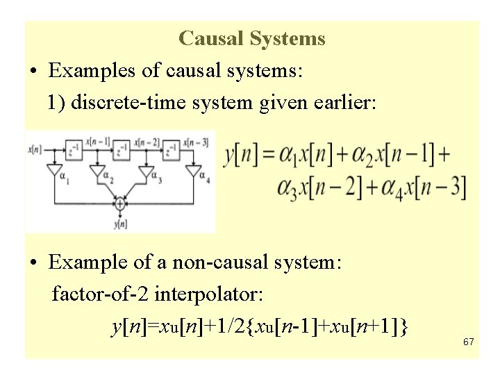
![Causal Systems • In a causal system, the n-th output sample y[n 0] depends Causal Systems • In a causal system, the n-th output sample y[n 0] depends](https://slidetodoc.com/presentation_image_h2/5502f711d94db79e3c52a97e07b4827b/image-66.jpg)
![Convolution and LTI System • From LTI system below, impulse response h[n] is simply Convolution and LTI System • From LTI system below, impulse response h[n] is simply](https://slidetodoc.com/presentation_image_h2/5502f711d94db79e3c52a97e07b4827b/image-69.jpg)
![• • Convolution and LTI System x[n] is a representation of linear combination • • Convolution and LTI System x[n] is a representation of linear combination](https://slidetodoc.com/presentation_image_h2/5502f711d94db79e3c52a97e07b4827b/image-70.jpg)
![Convolution and LTI System x[0]δ[n] x[0]h[n] x[1]δ[n-1] x[1]h[n-1] x[2]δ[n-2] x[2]h[n-2] x[l]δ[n-l] x[l]h[n-l] • The Convolution and LTI System x[0]δ[n] x[0]h[n] x[1]δ[n-1] x[1]h[n-1] x[2]δ[n-2] x[2]h[n-2] x[l]δ[n-l] x[l]h[n-l] • The](https://slidetodoc.com/presentation_image_h2/5502f711d94db79e3c52a97e07b4827b/image-72.jpg)
![Convolution and LTI System • Properties of the Convolution Sum: 1) Commutative property: x[n] Convolution and LTI System • Properties of the Convolution Sum: 1) Commutative property: x[n]](https://slidetodoc.com/presentation_image_h2/5502f711d94db79e3c52a97e07b4827b/image-73.jpg)
![Convolution and LTI System Computation of the Convolution Sum: • 1) Time-reverse h[k] to Convolution and LTI System Computation of the Convolution Sum: • 1) Time-reverse h[k] to](https://slidetodoc.com/presentation_image_h2/5502f711d94db79e3c52a97e07b4827b/image-74.jpg)
![Convolution and LTI System • Example: Develop the sequence y[n] generated by the convolution Convolution and LTI System • Example: Develop the sequence y[n] generated by the convolution](https://slidetodoc.com/presentation_image_h2/5502f711d94db79e3c52a97e07b4827b/image-78.jpg)
![Time-Domain Characterization of LTI Discrete-Time Systems • The sequence {y[n]} generated by the convolution Time-Domain Characterization of LTI Discrete-Time Systems • The sequence {y[n]} generated by the convolution](https://slidetodoc.com/presentation_image_h2/5502f711d94db79e3c52a97e07b4827b/image-80.jpg)
![Simple Interconnection Schemes of LTI Systems • Cascade Connection • Impulse response h[n] of Simple Interconnection Schemes of LTI Systems • Cascade Connection • Impulse response h[n] of](https://slidetodoc.com/presentation_image_h2/5502f711d94db79e3c52a97e07b4827b/image-84.jpg)
![Simple Interconnection Schemes of LTI Systems • Parallel Connection • Impulse response h[n] of Simple Interconnection Schemes of LTI Systems • Parallel Connection • Impulse response h[n] of](https://slidetodoc.com/presentation_image_h2/5502f711d94db79e3c52a97e07b4827b/image-86.jpg)
![Simple Interconnection Schemes of LTI Systems • Overall impulse response h[n] is given by: Simple Interconnection Schemes of LTI Systems • Overall impulse response h[n] is given by:](https://slidetodoc.com/presentation_image_h2/5502f711d94db79e3c52a97e07b4827b/image-89.jpg)
![Classification of LTI Discrete-Time Systems • The output y[n] of an FIR LTI discrete-time Classification of LTI Discrete-Time Systems • The output y[n] of an FIR LTI discrete-time](https://slidetodoc.com/presentation_image_h2/5502f711d94db79e3c52a97e07b4827b/image-94.jpg)
![Classification of LTI Discrete-Time Systems Based on Impulse Response Length • If h[n] is Classification of LTI Discrete-Time Systems Based on Impulse Response Length • If h[n] is](https://slidetodoc.com/presentation_image_h2/5502f711d94db79e3c52a97e07b4827b/image-96.jpg)
![Correlation of Signals • y[n] is said to be shifted by l samples to Correlation of Signals • y[n] is said to be shifted by l samples to](https://slidetodoc.com/presentation_image_h2/5502f711d94db79e3c52a97e07b4827b/image-101.jpg)
![Correlation of Signals • The autocorrelation sequence of x[n] is given by obtained by Correlation of Signals • The autocorrelation sequence of x[n] is given by obtained by](https://slidetodoc.com/presentation_image_h2/5502f711d94db79e3c52a97e07b4827b/image-102.jpg)
![Correlation of Signals • The cross-correlation of y[n] with the reference signal x[n] can Correlation of Signals • The cross-correlation of y[n] with the reference signal x[n] can](https://slidetodoc.com/presentation_image_h2/5502f711d94db79e3c52a97e07b4827b/image-104.jpg)
- Slides: 105

1. Time Domain Representation of Signals and Systems 1. 1 Discrete-Time Signals 1. 2 Operations on Sequences 1. 3 Classification of Sequences 1. 4 Some Basic Sequences 1. 5 The Sampling Process 1. 6 Discrete-Time Systems 1. 7 Classification of Discrete-Time Systems 1. 8 Time-Domain Characterization of LTI Systems 1. 9 Correlation 1

1. 1 Discrete-Time Signals • There are basically two types of discrete time signals: – Sampled-data signals in which samples are continuous-valued – digital signals in which samples are discrete-valued • Digital signals are obtained by quantizing the sample values either by rounding or truncation 2

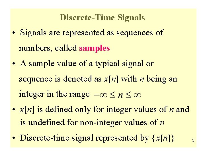
Discrete-Time Signals • Signals are represented as sequences of numbers, called samples • A sample value of a typical signal or sequence is denoted as x[n] with n being an integer in the range • x[n] is defined only for integer values of n and is undefined for non-integer values of n • Discrete-time signal represented by {x[n]} 3

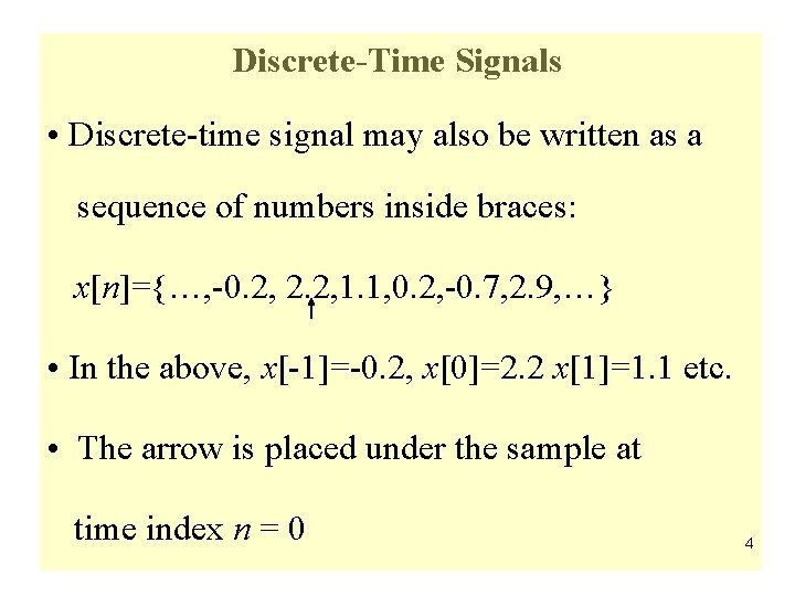
Discrete-Time Signals • Discrete-time signal may also be written as a sequence of numbers inside braces: x[n]={…, -0. 2, 2. 2, 1. 1, 0. 2, -0. 7, 2. 9, …} • In the above, x[-1]=-0. 2, x[0]=2. 2 x[1]=1. 1 etc. • The arrow is placed under the sample at time index n = 0 4

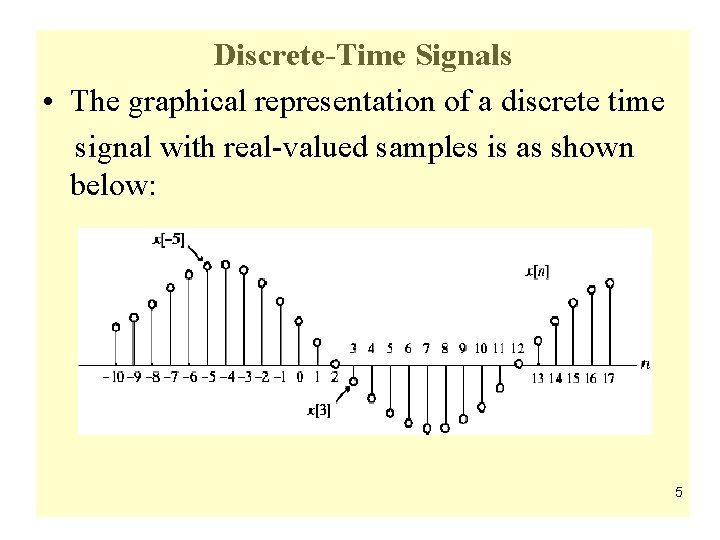
Discrete-Time Signals • The graphical representation of a discrete time signal with real-valued samples is as shown below: 5
![DiscreteTime Signals In some applications a discretetime sequence xn may be generated by Discrete-Time Signals • In some applications, a discrete-time sequence {x[n]} may be generated by](https://slidetodoc.com/presentation_image_h2/5502f711d94db79e3c52a97e07b4827b/image-6.jpg)
Discrete-Time Signals • In some applications, a discrete-time sequence {x[n]} may be generated by periodically sampling a continuous-time signal xa(t) at uniform time intervals 6
![DiscreteTime Signals Here nth sample is given by xn xattn T xan T Discrete-Time Signals • Here, n-th sample is given by: x[n]= xa(t)|t=n. T= xa(n. T),](https://slidetodoc.com/presentation_image_h2/5502f711d94db79e3c52a97e07b4827b/image-7.jpg)
Discrete-Time Signals • Here, n-th sample is given by: x[n]= xa(t)|t=n. T= xa(n. T), n=…, -2, -1, 0, 1, … • The spacing T between two consecutive samples is called the sampling interval or sampling period • Reciprocal of sampling interval T, denoted as FT is called sampling frequency: FT=1/T 7
![DiscreteTime Signals Whether or not the sequence xn has been obtained by sampling Discrete-Time Signals • Whether or not the sequence {x[n]} has been obtained by sampling,](https://slidetodoc.com/presentation_image_h2/5502f711d94db79e3c52a97e07b4827b/image-8.jpg)
Discrete-Time Signals • Whether or not the sequence {x[n]} has been obtained by sampling, the quantity, x[n] is called the n-th sample of the sequence • {x[n]} is a real sequence, if the n-th sample x[n] is real for all values of n • Otherwise, {x[n]} is a complex sequence 8
![DiscreteTime Signals A complex sequence xn can be written as xnxrenjximn where xren Discrete-Time Signals • A complex sequence {x[n]} can be written as {x[n]}={xre[n]+jxim[n]} where xre[n]](https://slidetodoc.com/presentation_image_h2/5502f711d94db79e3c52a97e07b4827b/image-9.jpg)
Discrete-Time Signals • A complex sequence {x[n]} can be written as {x[n]}={xre[n]+jxim[n]} where xre[n] and xim[n] are the real and imaginary parts of x[n] • The complex conjugate sequence of {x[n]} is given by {x*[n]}={xre[n]- jxim[n]} • Often the braces are ignored to denote a sequence if there is no ambiguity 9

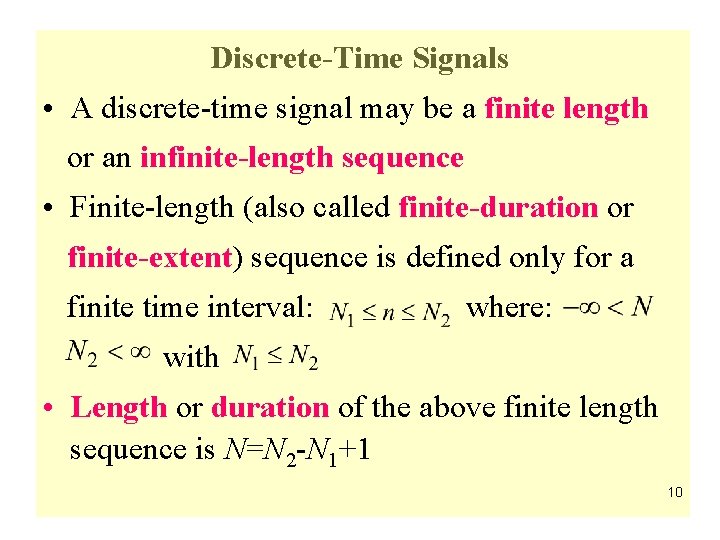
Discrete-Time Signals • A discrete-time signal may be a finite length or an infinite-length sequence • Finite-length (also called finite-duration or finite-extent) sequence is defined only for a finite time interval: where: with • Length or duration of the above finite length sequence is N=N 2 -N 1+1 10
![DiscreteTime Signals Examples xn n 2 is a finitelength sequence of length 8 Discrete-Time Signals • Examples: x[n]= n 2, is a finite-length sequence of length 8](https://slidetodoc.com/presentation_image_h2/5502f711d94db79e3c52a97e07b4827b/image-11.jpg)
Discrete-Time Signals • Examples: x[n]= n 2, is a finite-length sequence of length 8 y[n]=cos(0. 4 n) is an infinite-length sequence 11

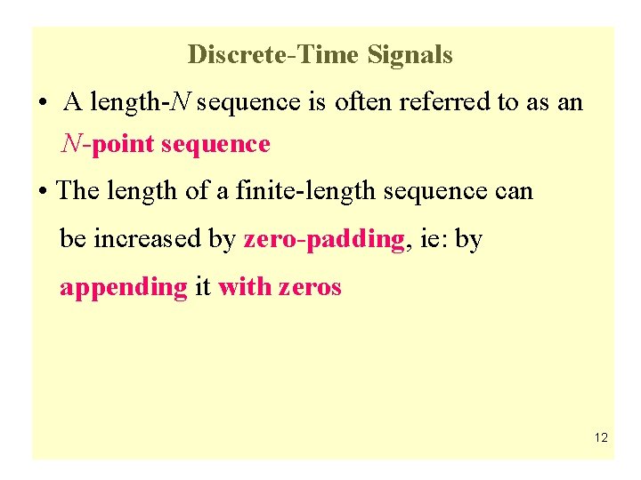
Discrete-Time Signals • A length-N sequence is often referred to as an N-point sequence • The length of a finite-length sequence can be increased by zero-padding, ie: by appending it with zeros 12

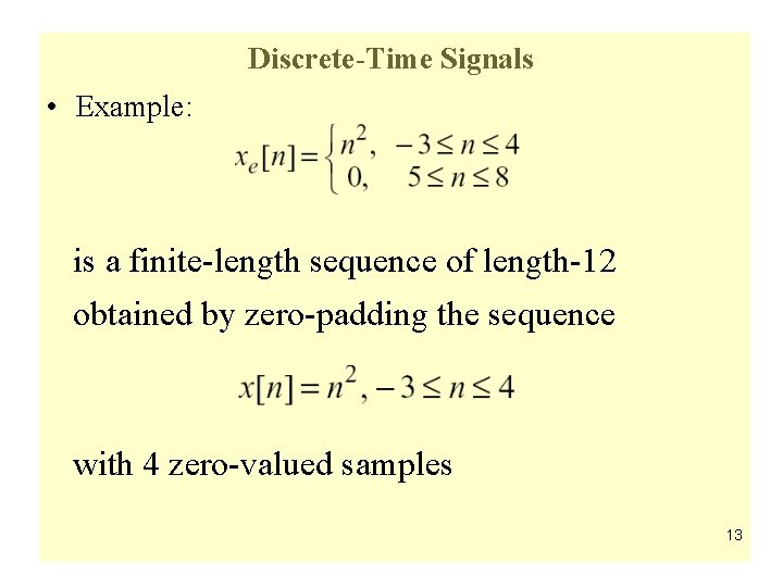
Discrete-Time Signals • Example: is a finite-length sequence of length-12 obtained by zero-padding the sequence with 4 zero-valued samples 13
![DiscreteTime Signals A rightsided sequence xn has zero valued samples for If Discrete-Time Signals • A right-sided sequence x[n] has zero valued samples for • If](https://slidetodoc.com/presentation_image_h2/5502f711d94db79e3c52a97e07b4827b/image-14.jpg)
Discrete-Time Signals • A right-sided sequence x[n] has zero valued samples for • If a right-sided sequence is called a causal sequence 14
![DiscreteTime Signals A leftsided sequence xn has zerovalued samples for If a Discrete-Time Signals • A left-sided sequence x[n] has zero-valued samples for • If a](https://slidetodoc.com/presentation_image_h2/5502f711d94db79e3c52a97e07b4827b/image-15.jpg)
Discrete-Time Signals • A left-sided sequence x[n] has zero-valued samples for • If a left-sided sequence is called a anti-causal sequence 15

1. 2 Operations on Sequences • A single-input, single-output discrete-time system operates on a sequence, called the input sequence, according some prescribed rules and develops another sequence, called the output sequence, with more desirable properties 16

Operations on Sequences • For example, the input may be a signal corrupted with additive noise • Discrete-time system is designed to generate an output by removing the noise component from the input • In most cases, the operation defining a particular discrete-time system is composed of some basic operations that we describe next: 17
![Basic Operations Product modulation operation ynxn wn Modulator An application is in Basic Operations • Product (modulation) operation: y[n]=x[n]. w[n] Modulator: • An application is in](https://slidetodoc.com/presentation_image_h2/5502f711d94db79e3c52a97e07b4827b/image-18.jpg)
Basic Operations • Product (modulation) operation: y[n]=x[n]. w[n] Modulator: • An application is in forming a finite-length sequence from an infinite-length sequence by multiplying with a window sequence • This process is usually called windowing 18
![Basic Operations Addition operation ynxnwn Adder Multiplication operation yn A xn Basic Operations • Addition operation: y[n]=x[n]+w[n] Adder: • Multiplication operation: y[n] = A. x[n]](https://slidetodoc.com/presentation_image_h2/5502f711d94db79e3c52a97e07b4827b/image-19.jpg)
Basic Operations • Addition operation: y[n]=x[n]+w[n] Adder: • Multiplication operation: y[n] = A. x[n] Multiplier: 19
![Basic Operations Timeshifting operation yn xn N where N is Basic Operations • Time-shifting operation: y[n] = x[n − N] , where N is](https://slidetodoc.com/presentation_image_h2/5502f711d94db79e3c52a97e07b4827b/image-20.jpg)
Basic Operations • Time-shifting operation: y[n] = x[n − N] , where N is an integer • If N > 0, it is delaying operation e. g. unit delay: y[n] = x[n − 1] • If N < 0, it is an advance operation, e. g. unit advance: y[n] = x[n +1] 20
![Basic Operations Timereversal operation yn xn Branching operation Used to provide Basic Operations • Time-reversal operation: y[n] = x[−n] • Branching operation: Used to provide](https://slidetodoc.com/presentation_image_h2/5502f711d94db79e3c52a97e07b4827b/image-21.jpg)
Basic Operations • Time-reversal operation: y[n] = x[−n] • Branching operation: Used to provide multiple copies of a sequence 21

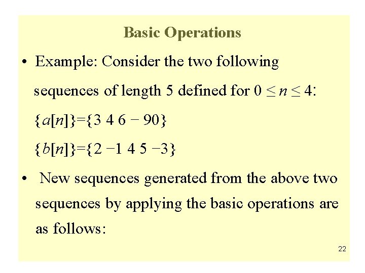
Basic Operations • Example: Consider the two following sequences of length 5 defined for 0 ≤ n ≤ 4: {a[n]}={3 4 6 − 90} {b[n]}={2 − 1 4 5 − 3} • New sequences generated from the above two sequences by applying the basic operations are as follows: 22
![Basic Operations cn anbn 6 4 24 450 dn an bn 5 Basic Operations {c[n]}= {a[n]⋅b[n]}= {6 − 4 24 − 450} {d[n]}= {a[n]+ b[n]}= {5](https://slidetodoc.com/presentation_image_h2/5502f711d94db79e3c52a97e07b4827b/image-23.jpg)
Basic Operations {c[n]}= {a[n]⋅b[n]}= {6 − 4 24 − 450} {d[n]}= {a[n]+ b[n]}= {5 3 10 − 4 − 3} {e[n]}={4. 5 6 9 13. 50} • As pointed out by the above examples, operations on two or more sequences can be carried out if all sequences involved are of same length and defined for the same range of the time index n 23

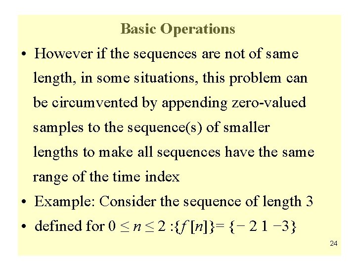
Basic Operations • However if the sequences are not of same length, in some situations, this problem can be circumvented by appending zero-valued samples to the sequence(s) of smaller lengths to make all sequences have the same range of the time index • Example: Consider the sequence of length 3 • defined for 0 ≤ n ≤ 2 : {f [n]}= {− 2 1 − 3} 24
![Basic Operations We cannot add the length3 sequence to the length5 sequence an Basic Operations • We cannot add the length-3 sequence to the length-5 sequence {a[n]}](https://slidetodoc.com/presentation_image_h2/5502f711d94db79e3c52a97e07b4827b/image-25.jpg)
Basic Operations • We cannot add the length-3 sequence to the length-5 sequence {a[n]} defined earlier • We therefore first append {f [n]} with 2 zero-valued samples resulting in a length-5 sequence {fe[n]}= {− 2 1 − 3 0 0} • Then {g[n]} ={a[n]}+{fe[n]} ={1 5 3 − 9 0} 25
![Combinations of Basic Operations Example yn α 1 xnα 2 xn 1α Combinations of Basic Operations • Example: y[n] =α 1 x[n]+α 2 x[n − 1]+α](https://slidetodoc.com/presentation_image_h2/5502f711d94db79e3c52a97e07b4827b/image-26.jpg)
Combinations of Basic Operations • Example: y[n] =α 1 x[n]+α 2 x[n − 1]+α 3 x[n − 2]+α 4 x[n − 3] 26
![1 3 Classification of Sequences Based on Symmetry Conjugatesymmetric sequence xn xn 1. 3 Classification of Sequences Based on Symmetry • Conjugate-symmetric sequence: x[n] = x*[−n]](https://slidetodoc.com/presentation_image_h2/5502f711d94db79e3c52a97e07b4827b/image-27.jpg)
1. 3 Classification of Sequences Based on Symmetry • Conjugate-symmetric sequence: x[n] = x*[−n] • If x[n] is real, then it is an even sequence An Even Sequence 27
![Classification of Sequences Based on Symmetry Conjugateantisymmetric sequence xn xn If Classification of Sequences Based on Symmetry • Conjugate-antisymmetric sequence: x[n] = −x*[−n] • If](https://slidetodoc.com/presentation_image_h2/5502f711d94db79e3c52a97e07b4827b/image-28.jpg)
Classification of Sequences Based on Symmetry • Conjugate-antisymmetric sequence: x[n] = −x*[−n] • If x[n] is real, then it is an odd sequence An Odd Sequence 28

Classification of Sequence Based on Symmetry • It follows from the definition that for a conjugate-symmetric sequence {x[n]}, x[0] must be a real number • Likewise, it follows from the definition that for a conjugate-antisymmetric sequence {y[n]}, y[0] must be an imaginary number • From the above, it also follows that for an odd sequence {w[n]}, w[0] = 0 29

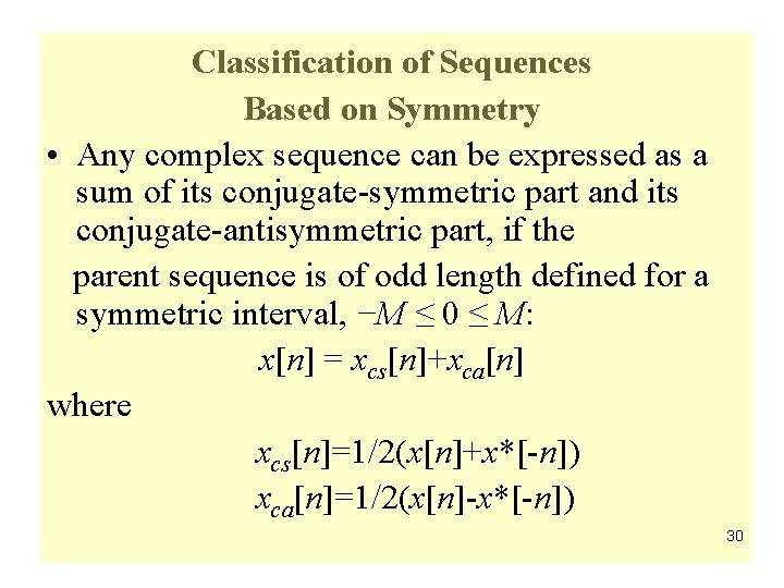
Classification of Sequences Based on Symmetry • Any complex sequence can be expressed as a sum of its conjugate-symmetric part and its conjugate-antisymmetric part, if the parent sequence is of odd length defined for a symmetric interval, −M ≤ 0 ≤ M: x[n] = xcs[n]+xca[n] where xcs[n]=1/2(x[n]+x*[-n]) xca[n]=1/2(x[n]-x*[-n]) 30

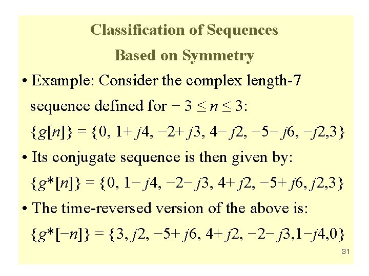
Classification of Sequences Based on Symmetry • Example: Consider the complex length-7 sequence defined for − 3 ≤ n ≤ 3: {g[n]} = {0, 1+ j 4, − 2+ j 3, 4− j 2, − 5− j 6, −j 2, 3} • Its conjugate sequence is then given by: {g*[n]} = {0, 1− j 4, − 2− j 3, 4+ j 2, − 5+ j 6, j 2, 3} • The time-reversed version of the above is: {g*[−n]} = {3, j 2, − 5+ j 6, 4+ j 2, − 2− j 3, 1−j 4, 0} 31
![Classification of Sequences Based on Symmetry Therefore gcsn12gn g n 1 5 0 Classification of Sequences Based on Symmetry • Therefore {gcs[n]}=1/2{g[n]+ g *[−n]} ={1. 5, 0.](https://slidetodoc.com/presentation_image_h2/5502f711d94db79e3c52a97e07b4827b/image-32.jpg)
Classification of Sequences Based on Symmetry • Therefore {gcs[n]}=1/2{g[n]+ g *[−n]} ={1. 5, 0. 5+ j 3, − 3. 5+ j 4. 5, 4, − 3. 5− j 4. 5, 0. 5− j 3, 1. 5} • Likewise {gca[n]}=1/2 {g[n]− g *[−n]} ={− 1. 5, 0. 5+ j, 1. 5− j 1. 5, − j 2, − 1. 5− j 1. 5, − 0. 5− j, 1. 5} • It can be easily verified that gcs[n]= gcs*[-n]= and gca[n] = − gca*[-n] 32
![Classification of Sequences Periodic and Aperiodic Signals A sequence xn satisfying xnxnk N Classification of Sequences: Periodic and Aperiodic Signals • A sequence x[n] satisfying: x[n]=x[n+k. N]](https://slidetodoc.com/presentation_image_h2/5502f711d94db79e3c52a97e07b4827b/image-33.jpg)
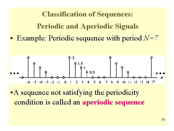
Classification of Sequences: Periodic and Aperiodic Signals • A sequence x[n] satisfying: x[n]=x[n+k. N] is called a periodic sequence with a period N where N is a positive integer and k is any integer • Smallest value of N satisfying x[n]=x[n+k. N] is called the fundamental period 33

Classification of Sequences: Periodic and Aperiodic Signals • Example: Periodic sequence with period N=7 • A sequence not satisfying the periodicity condition is called an aperiodic sequence 34

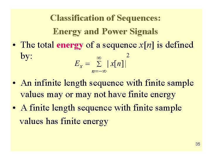
Classification of Sequences: Energy and Power Signals • The total energy of a sequence x[n] is defined by: • An infinite length sequence with finite sample values may or may not have finite energy • A finite length sequence with finite sample values has finite energy 35

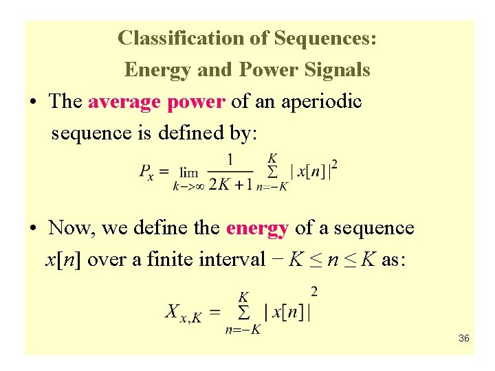
Classification of Sequences: Energy and Power Signals • The average power of an aperiodic sequence is defined by: • Now, we define the energy of a sequence x[n] over a finite interval − K ≤ n ≤ K as: 36

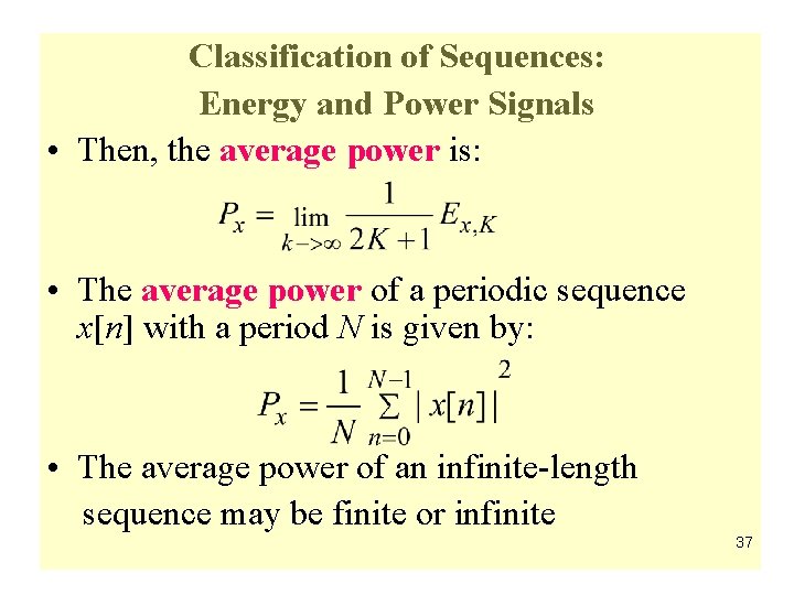
Classification of Sequences: Energy and Power Signals • Then, the average power is: • The average power of a periodic sequence x[n] with a period N is given by: • The average power of an infinite-length sequence may be finite or infinite 37

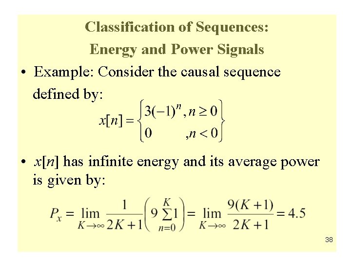
Classification of Sequences: Energy and Power Signals • Example: Consider the causal sequence defined by: • x[n] has infinite energy and its average power is given by: 38

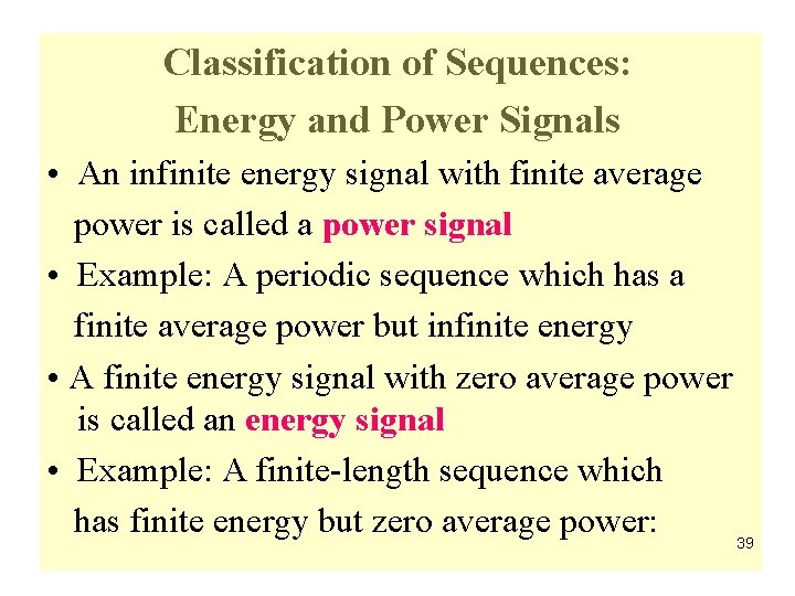
Classification of Sequences: Energy and Power Signals • An infinite energy signal with finite average power is called a power signal • Example: A periodic sequence which has a finite average power but infinite energy • A finite energy signal with zero average power is called an energy signal • Example: A finite-length sequence which has finite energy but zero average power: 39
![Classification of Sequences Other Types of Classifications A sequence xn is said to Classification of Sequences: Other Types of Classifications • A sequence x[n] is said to](https://slidetodoc.com/presentation_image_h2/5502f711d94db79e3c52a97e07b4827b/image-40.jpg)
Classification of Sequences: Other Types of Classifications • A sequence x[n] is said to be bounded if each of its samples is of magnitude less than or equal to a finite positive number Bx, i. e. , • Example: The sequence x[n]=cos(0. 3πn) is a bounded sequence as: |x[n]| = |cos 0. 3πn| ≤ 1 40
![Classification of Sequences Other Types of Classifications A sequence xn is said to Classification of Sequences: Other Types of Classifications • A sequence x[n] is said to](https://slidetodoc.com/presentation_image_h2/5502f711d94db79e3c52a97e07b4827b/image-41.jpg)
Classification of Sequences: Other Types of Classifications • A sequence x[n] is said to be absolutely summable if: Example: is an absolutely summable sequence as: 41

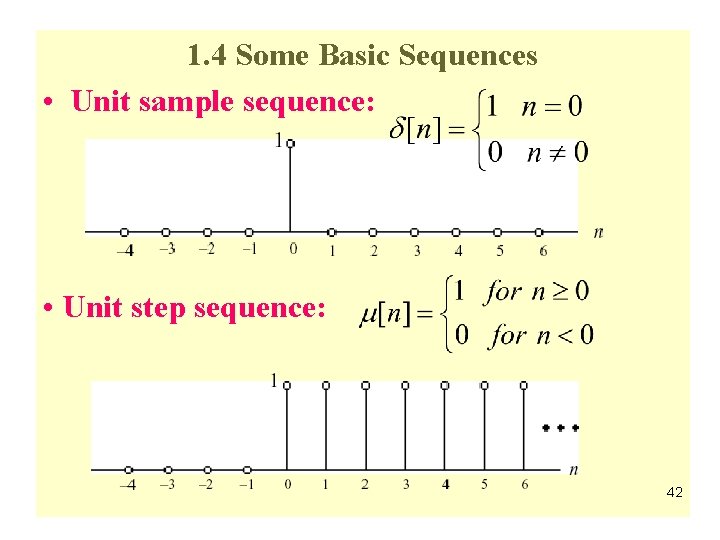
1. 4 Some Basic Sequences • Unit sample sequence: • Unit step sequence: 42

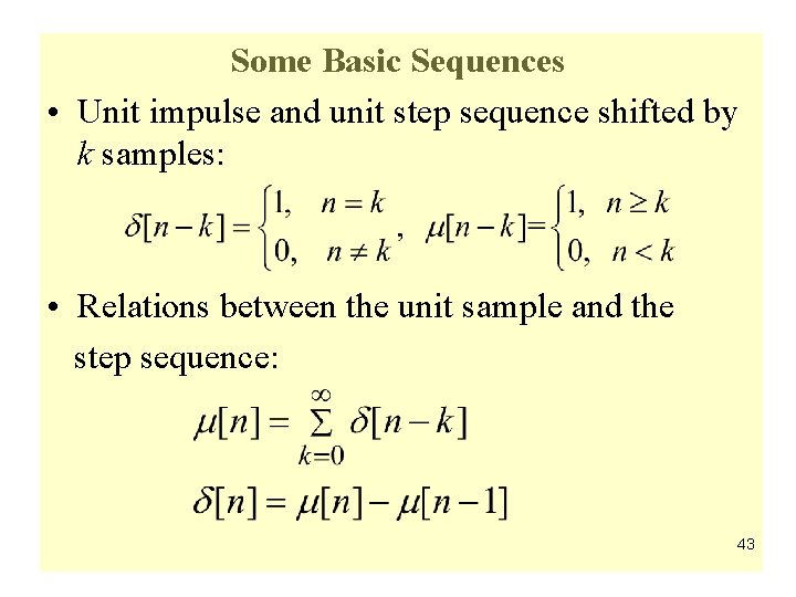
Some Basic Sequences • Unit impulse and unit step sequence shifted by k samples: • Relations between the unit sample and the step sequence: 43
![Some Basic Sequences Real sinusoidal sequence xn Asinωon φ where A Some Basic Sequences • Real sinusoidal sequence: x[n] = Asin(ωon + φ) where A](https://slidetodoc.com/presentation_image_h2/5502f711d94db79e3c52a97e07b4827b/image-44.jpg)
Some Basic Sequences • Real sinusoidal sequence: x[n] = Asin(ωon + φ) where A is the amplitude, ωo is the angular frequency, and is the phase of x[n] • Example: 44
![Some Basic Sequences Exponential sequence xn Aαn n Some Basic Sequences • Exponential sequence: x[n] = Aαn , − ∞ < n](https://slidetodoc.com/presentation_image_h2/5502f711d94db79e3c52a97e07b4827b/image-45.jpg)
Some Basic Sequences • Exponential sequence: x[n] = Aαn , − ∞ < n < ∞ where A and α are real or complex numbers • If we write: then we can express: where: 45
![Some Basic Sequences x n of a complex exponential sequence are real sinusoidal Some Basic Sequences • x [n] of a complex exponential sequence are real sinusoidal](https://slidetodoc.com/presentation_image_h2/5502f711d94db79e3c52a97e07b4827b/image-46.jpg)
Some Basic Sequences • x [n] of a complex exponential sequence are real sinusoidal sequences with constant (σo= 0), growing (σo > 0) or decaying (σo < 0) amplitudes for n > 0 • Example: x[n] exp(-1/12+jπ/6)n 46
![Some Basic Sequences Real exponential sequence xn Aαn n Some Basic Sequences • Real exponential sequence: x[n] =Aαn, −∞ < n < ∞](https://slidetodoc.com/presentation_image_h2/5502f711d94db79e3c52a97e07b4827b/image-47.jpg)
Some Basic Sequences • Real exponential sequence: x[n] =Aαn, −∞ < n < ∞ where A and α are real numbers. Example: 47

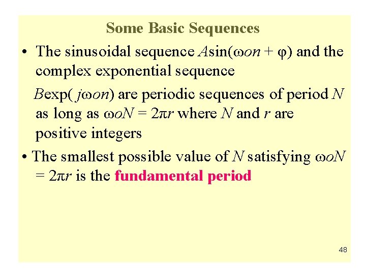
Some Basic Sequences • The sinusoidal sequence Asin(ωon + φ) and the complex exponential sequence Bexp( jωon) are periodic sequences of period N as long as ωo. N = 2πr where N and r are positive integers • The smallest possible value of N satisfying ωo. N = 2πr is the fundamental period 48

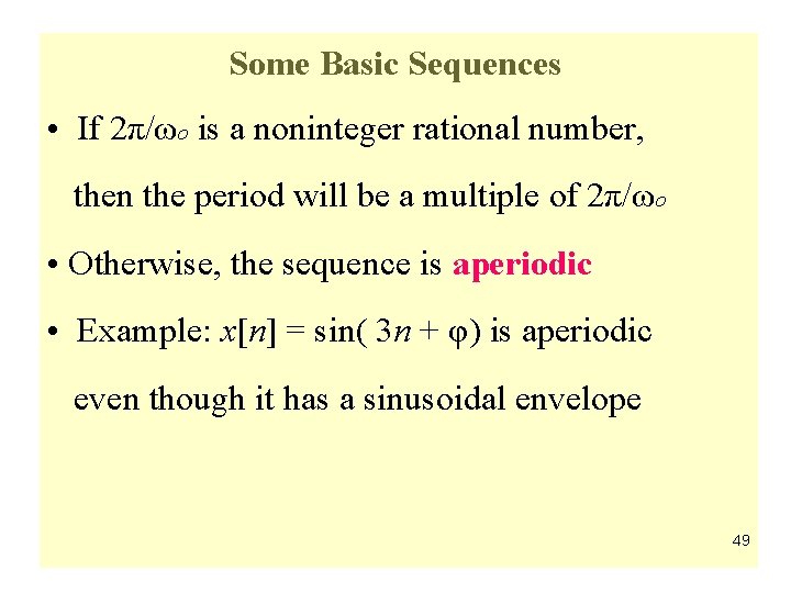
Some Basic Sequences • If 2π/ωo is a noninteger rational number, then the period will be a multiple of 2π/ωo • Otherwise, the sequence is aperiodic • Example: x[n] = sin( 3 n + φ) is aperiodic even though it has a sinusoidal envelope 49

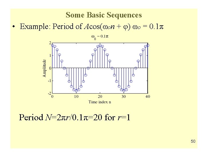
Some Basic Sequences • Example: Period of Acos(ωon + φ) ωo = 0. 1π Period N=2πr/0. 1π=20 for r=1 50

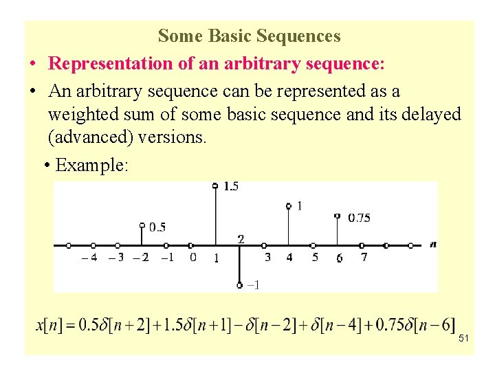
Some Basic Sequences • Representation of an arbitrary sequence: • An arbitrary sequence can be represented as a weighted sum of some basic sequence and its delayed (advanced) versions. • Example: 51
![1 5 The Sampling Process Often a sequence xn is developed by sampling 1. 5 The Sampling Process • Often, a sequence x[n] is developed by sampling](https://slidetodoc.com/presentation_image_h2/5502f711d94db79e3c52a97e07b4827b/image-52.jpg)
1. 5 The Sampling Process • Often, a sequence x[n] is developed by sampling a continuous-time signal xa(t) • The relation between the two signals is: 52

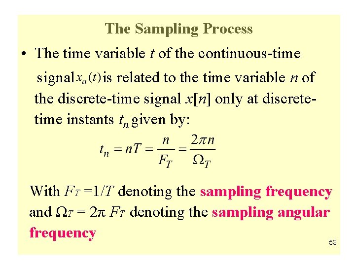
The Sampling Process • The time variable t of the continuous-time signal is related to the time variable n of the discrete-time signal x[n] only at discretetime instants tn given by: With FT =1/T denoting the sampling frequency and ΩT = 2π FT denoting the sampling angular frequency 53

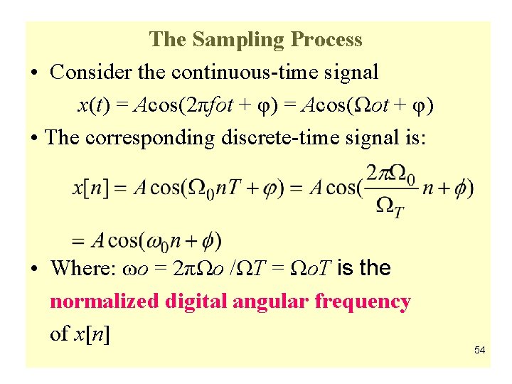
The Sampling Process • Consider the continuous-time signal x(t) = Acos(2πfot + φ) = Acos(Ωot + φ) • The corresponding discrete-time signal is: • Where: ωo = 2πΩo /ΩT = Ωo. T is the normalized digital angular frequency of x[n] 54

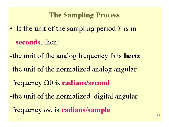
The Sampling Process • If the unit of the sampling period T is in seconds, then: -the unit of the analog frequency f 0 is hertz -the unit of the normalized analog angular frequency Ω 0 is radians/second -the unit of the normalized digital angular frequency ωo is radians/sample 55
![The Sampling Process Example Determine the discretetime signal vn obtained by uniformly sampling The Sampling Process • Example: Determine the discrete-time signal v[n] obtained by uniformly sampling](https://slidetodoc.com/presentation_image_h2/5502f711d94db79e3c52a97e07b4827b/image-56.jpg)
The Sampling Process • Example: Determine the discrete-time signal v[n] obtained by uniformly sampling at a sampling rate of 200 Hz the continuous time signal: v(t)=6 cos(60πt)+2 cos(100 πt)+10 sin(140 πt) composed of a weighted sum of 3 sinusoidal signals of frequencies 30 Hz, 50 Hz, and 70 Hz 56
![1 6 DiscreteTime Systems A discretetime system processes a given input sequence xn 1. 6 Discrete-Time Systems • A discrete-time system processes a given input sequence x[n]](https://slidetodoc.com/presentation_image_h2/5502f711d94db79e3c52a97e07b4827b/image-57.jpg)
1. 6 Discrete-Time Systems • A discrete-time system processes a given input sequence x[n] to generates an output sequence y[n] with more desirable properties • In most applications, the discrete-time system is a single-input, single-output system: 57

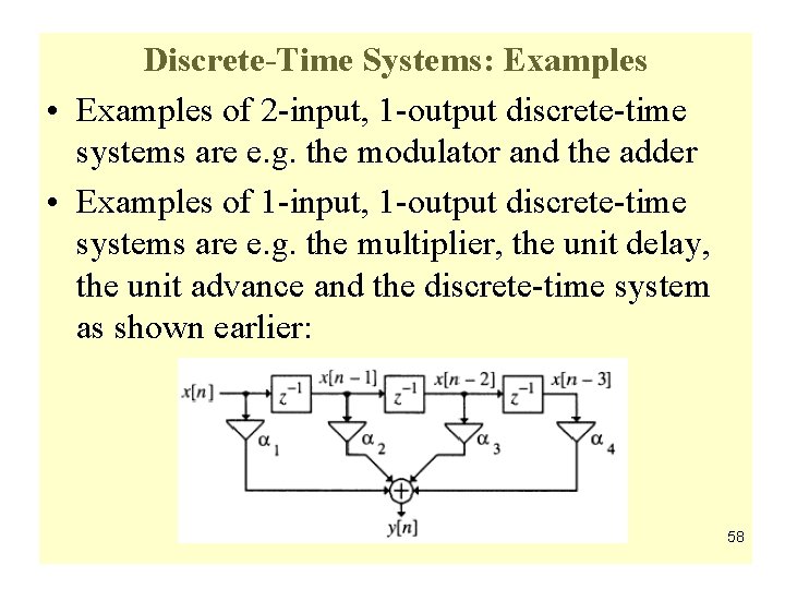
Discrete-Time Systems: Examples • Examples of 2 -input, 1 -output discrete-time systems are e. g. the modulator and the adder • Examples of 1 -input, 1 -output discrete-time systems are e. g. the multiplier, the unit delay, the unit advance and the discrete-time system as shown earlier: 58

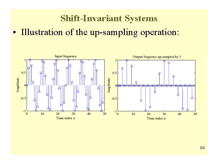
Discrete-Time Systems: Examples • Up-sampling– process of increasing the sampling rate of a signal. Eg Application: Up-sampling image data such as photograph means increase the resolution of the photograph. • Down-Sampling-also known as sub-sampling means process of reducing the sampling rate of a signal Eg Application: Down-sampling to reduce the data rate or the size of the data 59

1. 7 Classification of Discrete-Time Systems • Classification of discrete-time systems: -Linear Systems -Shift-Invariant Systems -Causal Systems -Stable Systems -Passive and Lossless Systems 60
![Linear Systems Linear systems have the property that if x 1n y 1n Linear Systems • Linear systems have the property that if: x 1[n] y 1[n]](https://slidetodoc.com/presentation_image_h2/5502f711d94db79e3c52a97e07b4827b/image-61.jpg)
Linear Systems • Linear systems have the property that if: x 1[n] y 1[n] and x 2[n] y 2[n] , then: x[n]=αx 1[n]+ßx 2[n] y[n]= αy 1[n]+ßy 2[n] • If input consists of a sum of scaled sequences, then the corresponding output is a sum of scaled outputs corresponding to the individual input sequences 61
![α x 1n y 1n wn X System x 2n System y 2n α x 1[n] y 1[n] w[n] X System + x 2[n] System y 2[n]](https://slidetodoc.com/presentation_image_h2/5502f711d94db79e3c52a97e07b4827b/image-62.jpg)
α x 1[n] y 1[n] w[n] X System + x 2[n] System y 2[n] X ß x 1[n] X w[n]=y[n] when system is linear! α + x[n] System y[n] x 2[n] X ß 62

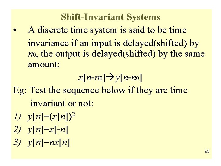
Shift-Invariant Systems • A discrete time system is said to be time invariance if an input is delayed(shifted) by n 0, the output is delayed(shifted) by the same amount: x[n-n 0] y[n-n 0] Eg: Test the sequence below if they are time invariant or not: 1) y[n]=(x[n])2 2) y[n]=x[-n] 3) y[n]=nx[n] 63

Shift-Invariant Systems • Illustration of the up-sampling operation: 64

• • • Linear Time-Invariant Systems Linear Time-Invariant (LTI) System: A system satisfying both the linearity and the time-invariance property is called a LTI systems are mathematically easy to analyze and characterize, and consequently, easy to design Highly useful signal processing algorithms have been developed utilizing this class of systems over the last several decades 65
![Causal Systems In a causal system the nth output sample yn 0 depends Causal Systems • In a causal system, the n-th output sample y[n 0] depends](https://slidetodoc.com/presentation_image_h2/5502f711d94db79e3c52a97e07b4827b/image-66.jpg)
Causal Systems • In a causal system, the n-th output sample y[n 0] depends only on input samples x[n] for n ≤ no and does not depend on input samples for n > no • Simply speaking, for a causal system, changes in output samples do not precede changes in the input samples 66

Causal Systems • Examples of causal systems: 1) discrete-time system given earlier: • Example of a non-causal system: factor-of-2 interpolator: y[n]=xu[n]+1/2{xu[n-1]+xu[n+1]} 67

Stable Systems • There are various definitions of stability • We consider here the bounded-input, bounded-output (BIBO) stability • If y[n] is the response to an input x[n] and if: |x[n]|≤Bx for all values of n, then: |y[n]|≤By for all values of n, where Bx and By are finite constants 68
![Convolution and LTI System From LTI system below impulse response hn is simply Convolution and LTI System • From LTI system below, impulse response h[n] is simply](https://slidetodoc.com/presentation_image_h2/5502f711d94db79e3c52a97e07b4827b/image-69.jpg)
Convolution and LTI System • From LTI system below, impulse response h[n] is simply the output when the input is unit impulse sequence δ[n] • Any signal x[n] can be represented as sum of scaled and shifted impulse signals: 69
![Convolution and LTI System xn is a representation of linear combination • • Convolution and LTI System x[n] is a representation of linear combination](https://slidetodoc.com/presentation_image_h2/5502f711d94db79e3c52a97e07b4827b/image-70.jpg)
• • Convolution and LTI System x[n] is a representation of linear combination of scaled, shifted impulses. Since LTI systems respond in simple and predictable ways to sum of signals and to shifted signals, this representation is particularly useful for deriving a general formula of LTI system From figure, response to input δ[n] is by definition the impulse response h[n] Time Invariance gives information response due to δ[n-1] is h[n-1] 70

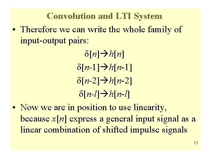
Convolution and LTI System • Therefore we can write the whole family of input-output pairs: δ[n] h[n] δ[n-1] h[n-1] δ[n-2] h[n-2] δ[n-l] h[n-l] • Now we are in position to use linearity, because x[n] express a general input signal as a linear combination of shifted impulse signals 71
![Convolution and LTI System x0δn x0hn x1δn1 x1hn1 x2δn2 x2hn2 xlδnl xlhnl The Convolution and LTI System x[0]δ[n] x[0]h[n] x[1]δ[n-1] x[1]h[n-1] x[2]δ[n-2] x[2]h[n-2] x[l]δ[n-l] x[l]h[n-l] • The](https://slidetodoc.com/presentation_image_h2/5502f711d94db79e3c52a97e07b4827b/image-72.jpg)
Convolution and LTI System x[0]δ[n] x[0]h[n] x[1]δ[n-1] x[1]h[n-1] x[2]δ[n-2] x[2]h[n-2] x[l]δ[n-l] x[l]h[n-l] • The we use superposition to put it all together: CONVOLUTION SUM OR 72
![Convolution and LTI System Properties of the Convolution Sum 1 Commutative property xn Convolution and LTI System • Properties of the Convolution Sum: 1) Commutative property: x[n]](https://slidetodoc.com/presentation_image_h2/5502f711d94db79e3c52a97e07b4827b/image-73.jpg)
Convolution and LTI System • Properties of the Convolution Sum: 1) Commutative property: x[n] * h[n] = h[n] * x[n] 2) Associative property: (x[n] * h[n]) * y[n] = x[n] * (h[n] * y[n]) 3) Distributive property: x[n] * (h[n] + y[n]) = x[n] * h[n] + x[n] * y[n] 73
![Convolution and LTI System Computation of the Convolution Sum 1 Timereverse hk to Convolution and LTI System Computation of the Convolution Sum: • 1) Time-reverse h[k] to](https://slidetodoc.com/presentation_image_h2/5502f711d94db79e3c52a97e07b4827b/image-74.jpg)
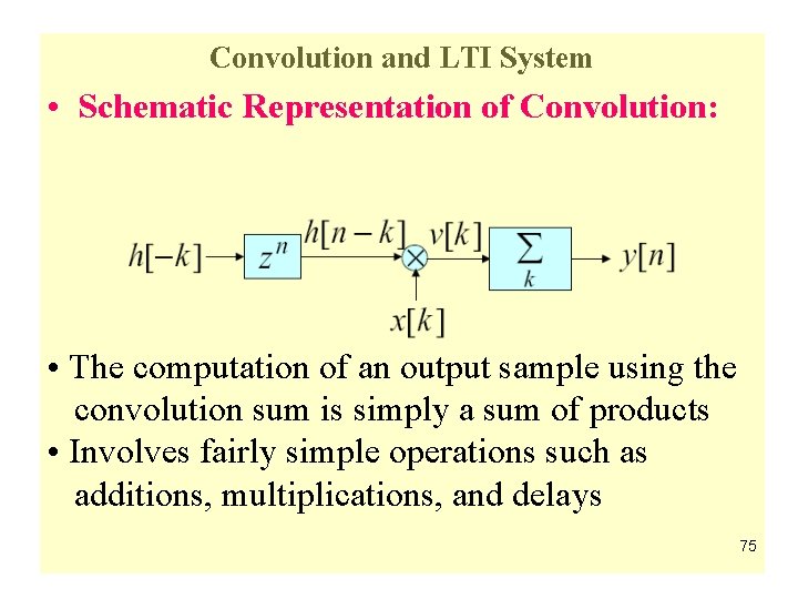
Convolution and LTI System Computation of the Convolution Sum: • 1) Time-reverse h[k] to form h[−k] • 2) Shift h[−k] to the right by n sampling periods if n > 0 or shift to the left by n sampling periods if n < 0 to form h[n − k] • 3) Form the product v[k] = x[k]h[n − k] • 4) Sum all samples of v[k] to develop the n-th sample of y[n] of the convolution sum 74

Convolution and LTI System • Schematic Representation of Convolution: • The computation of an output sample using the convolution sum is simply a sum of products • Involves fairly simple operations such as additions, multiplications, and delays 75

Convolution and LTI System • In practice, if either the input or the impulse response is of finite length, the convolution sum can be used to compute the output sample as it involves a finite sum of products • If both the input sequence and the impulse response sequence are of finite length, the output sequence is also of finite length 76

Convolution and LTI System • If both the input sequence and the impulse response sequence are of infinite length, the convolution sum cannot be used to compute the output • For systems characterized by an infinite impulse response sequence, an alternate time-domain description involving a finite sum of products will be considered 77
![Convolution and LTI System Example Develop the sequence yn generated by the convolution Convolution and LTI System • Example: Develop the sequence y[n] generated by the convolution](https://slidetodoc.com/presentation_image_h2/5502f711d94db79e3c52a97e07b4827b/image-78.jpg)
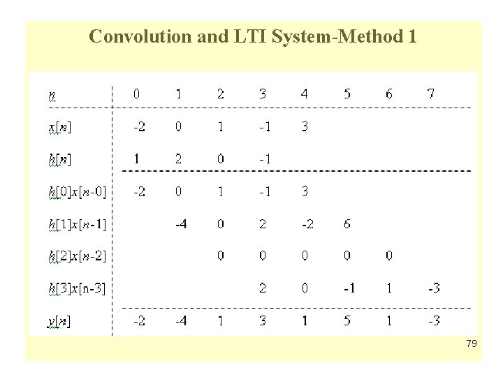
Convolution and LTI System • Example: Develop the sequence y[n] generated by the convolution of the sequences x[n] and h[n] shown below 78

Convolution and LTI System-Method 1 79
![TimeDomain Characterization of LTI DiscreteTime Systems The sequence yn generated by the convolution Time-Domain Characterization of LTI Discrete-Time Systems • The sequence {y[n]} generated by the convolution](https://slidetodoc.com/presentation_image_h2/5502f711d94db79e3c52a97e07b4827b/image-80.jpg)
Time-Domain Characterization of LTI Discrete-Time Systems • The sequence {y[n]} generated by the convolution sum is shown below: 80

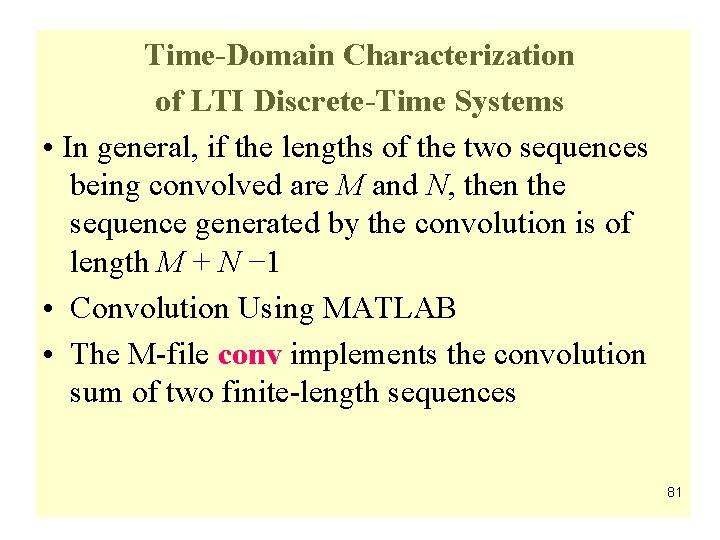
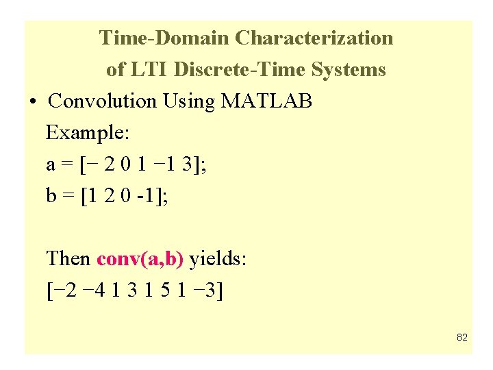
Time-Domain Characterization of LTI Discrete-Time Systems • In general, if the lengths of the two sequences being convolved are M and N, then the sequence generated by the convolution is of length M + N − 1 • Convolution Using MATLAB • The M-file conv implements the convolution sum of two finite-length sequences 81

Time-Domain Characterization of LTI Discrete-Time Systems • Convolution Using MATLAB Example: a = [− 2 0 1 − 1 3]; b = [1 2 0 -1]; Then conv(a, b) yields: [− 2 − 4 1 3 1 5 1 − 3] 82

Simple Interconnection Schemes of LTI Systems • Two simple interconnection schemes of LTI systems are: 1) Cascade Connection 2) Parallel Connection • They are widely used for developing complex LTI systems from simple LTI system sections 83
![Simple Interconnection Schemes of LTI Systems Cascade Connection Impulse response hn of Simple Interconnection Schemes of LTI Systems • Cascade Connection • Impulse response h[n] of](https://slidetodoc.com/presentation_image_h2/5502f711d94db79e3c52a97e07b4827b/image-84.jpg)
Simple Interconnection Schemes of LTI Systems • Cascade Connection • Impulse response h[n] of the cascade of two LTI discrete time systems with impulse responses h 1[n] and h 2[n] is given by: h[n] = h 1[n] * h 2[n] 84

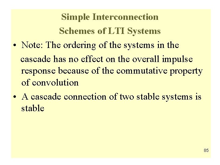
Simple Interconnection Schemes of LTI Systems • Note: The ordering of the systems in the cascade has no effect on the overall impulse response because of the commutative property of convolution • A cascade connection of two stable systems is stable 85
![Simple Interconnection Schemes of LTI Systems Parallel Connection Impulse response hn of Simple Interconnection Schemes of LTI Systems • Parallel Connection • Impulse response h[n] of](https://slidetodoc.com/presentation_image_h2/5502f711d94db79e3c52a97e07b4827b/image-86.jpg)
Simple Interconnection Schemes of LTI Systems • Parallel Connection • Impulse response h[n] of the parallel connection of two LTI discrete-time systems with impulse responses h 1[n] and h 2[n] is given by: 86 h[n]=h 1[n]+h 2[n]

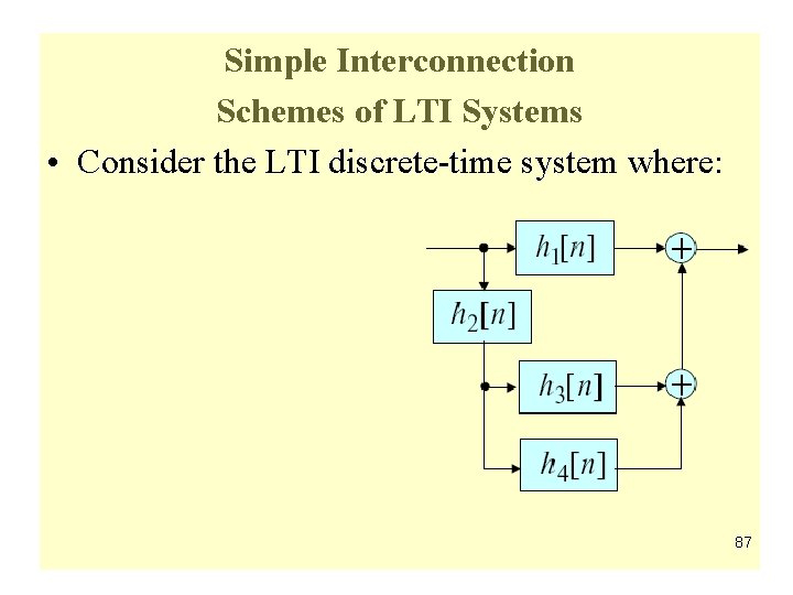
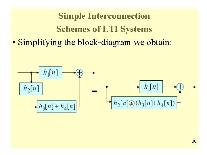
Simple Interconnection Schemes of LTI Systems • Consider the LTI discrete-time system where: 87

Simple Interconnection Schemes of LTI Systems • Simplifying the block-diagram we obtain: 88
![Simple Interconnection Schemes of LTI Systems Overall impulse response hn is given by Simple Interconnection Schemes of LTI Systems • Overall impulse response h[n] is given by:](https://slidetodoc.com/presentation_image_h2/5502f711d94db79e3c52a97e07b4827b/image-89.jpg)
Simple Interconnection Schemes of LTI Systems • Overall impulse response h[n] is given by: h[n] = h 1[n]+ h 2[n] * (h 3[n]+h 4[n]) = h 1[n]+ h 2[n]*h 3[n]+h 2[n]*h 4[n] • Now: 89

Simple Interconnection Schemes of LTI Systems 90

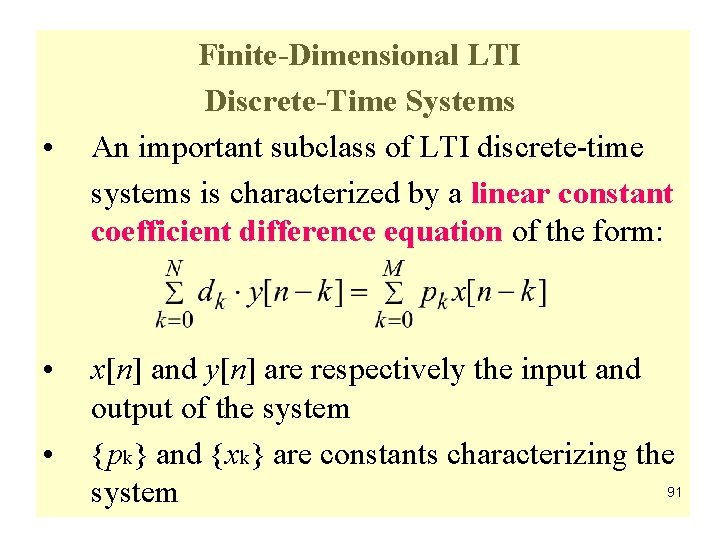
• • • Finite-Dimensional LTI Discrete-Time Systems An important subclass of LTI discrete-time systems is characterized by a linear constant coefficient difference equation of the form: x[n] and y[n] are respectively the input and output of the system {pk} and {xk} are constants characterizing the 91 system

Finite-Dimensional LTI Discrete-Time Systems • The order of the LTI system is given by max(N, M), which is the order of the difference equation • It is possible to implement an LTI system characterized by a constant coefficient difference equation as here the computation involves two finite sums of products even though such a system, in general, has an impulse response of infinite length 92

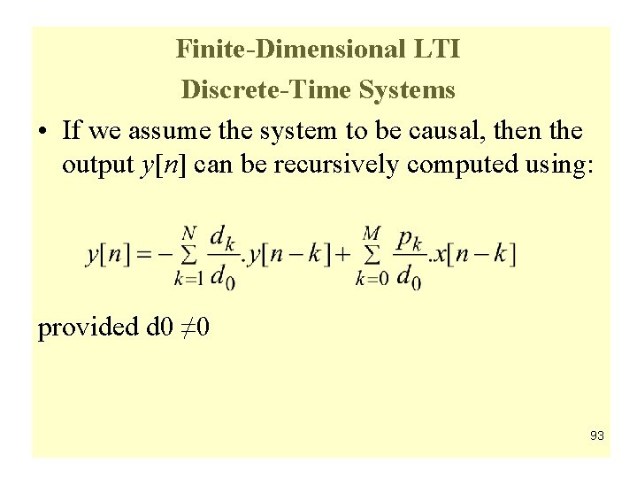
Finite-Dimensional LTI Discrete-Time Systems • If we assume the system to be causal, then the output y[n] can be recursively computed using: provided d 0 ≠ 0 93
![Classification of LTI DiscreteTime Systems The output yn of an FIR LTI discretetime Classification of LTI Discrete-Time Systems • The output y[n] of an FIR LTI discrete-time](https://slidetodoc.com/presentation_image_h2/5502f711d94db79e3c52a97e07b4827b/image-94.jpg)
Classification of LTI Discrete-Time Systems • The output y[n] of an FIR LTI discrete-time system can be computed directly from the convolution sum as it is a finite sum of products • Examples of FIR LTI discrete-time systems are the moving-average system and the linear interpolators 94

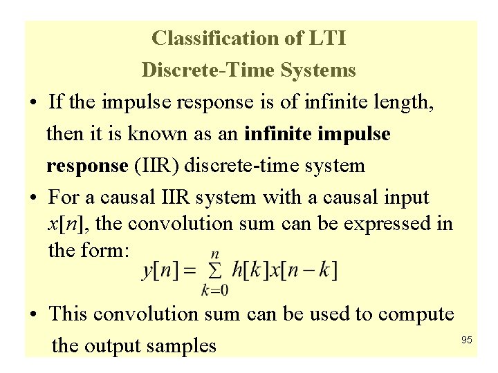
Classification of LTI Discrete-Time Systems • If the impulse response is of infinite length, then it is known as an infinite impulse response (IIR) discrete-time system • For a causal IIR system with a causal input x[n], the convolution sum can be expressed in the form: • This convolution sum can be used to compute the output samples 95
![Classification of LTI DiscreteTime Systems Based on Impulse Response Length If hn is Classification of LTI Discrete-Time Systems Based on Impulse Response Length • If h[n] is](https://slidetodoc.com/presentation_image_h2/5502f711d94db79e3c52a97e07b4827b/image-96.jpg)
Classification of LTI Discrete-Time Systems Based on Impulse Response Length • If h[n] is of finite length, Eg: h[n] = 0 for n < N 1 and n > N 2, N 1 < N 2 then it is known as a finite impulse response (FIR) discrete-time system • The convolution sum reduces to: 96

Classification of LTI Discrete-Time Systems Based on the Output Calculation Process • Nonrecursive System: Here the output can be calculated sequentially, knowing only the present and past input samples • Recursive System: Here the output computation involves past output samples in addition to the present and past input samples 97

Correlation of Signals • There applications where it is necessary to compare one reference signal with one or more signals to determine the similarity between the pair and to determine additional information based on the similarity 98

Correlation of Signals • Example: In radar and sonar applications, the received signal reflected from the target is the delayed version of the transmitted signal and by measuring the delay, one can determine the location of the target • The detection problem gets more complicated in practice, as often the received signal is corrupted by additive random noise 99

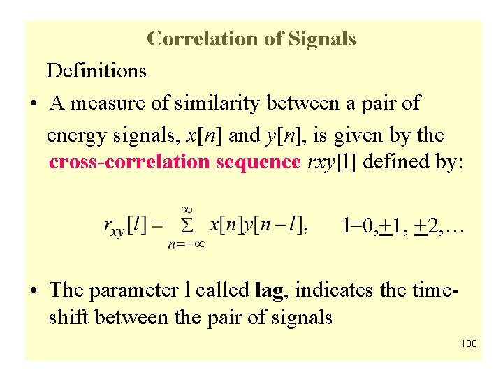
Correlation of Signals Definitions • A measure of similarity between a pair of energy signals, x[n] and y[n], is given by the cross-correlation sequence rxy[l] defined by: l=0, +1, +2, … • The parameter l called lag, indicates the timeshift between the pair of signals 100
![Correlation of Signals yn is said to be shifted by l samples to Correlation of Signals • y[n] is said to be shifted by l samples to](https://slidetodoc.com/presentation_image_h2/5502f711d94db79e3c52a97e07b4827b/image-101.jpg)
Correlation of Signals • y[n] is said to be shifted by l samples to the right with respect to the reference sequence x[n] for positive values of l, and shifted by l samples to the left for negative values of l • The ordering of the subscripts xy in the definition of rxy[l] specifies that x[n] is the reference sequence which remains fixed in time while y[n] is being shifted with respect to x[n] 101
![Correlation of Signals The autocorrelation sequence of xn is given by obtained by Correlation of Signals • The autocorrelation sequence of x[n] is given by obtained by](https://slidetodoc.com/presentation_image_h2/5502f711d94db79e3c52a97e07b4827b/image-102.jpg)
Correlation of Signals • The autocorrelation sequence of x[n] is given by obtained by setting y[n] = x[n] in the above definition of the cross-correlation sequence rxy[l] 102

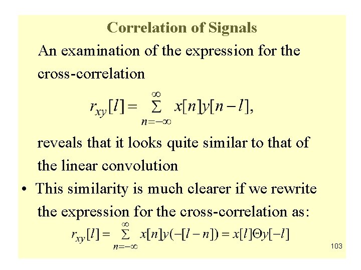
Correlation of Signals An examination of the expression for the cross-correlation reveals that it looks quite similar to that of the linear convolution • This similarity is much clearer if we rewrite the expression for the cross-correlation as: 103
![Correlation of Signals The crosscorrelation of yn with the reference signal xn can Correlation of Signals • The cross-correlation of y[n] with the reference signal x[n] can](https://slidetodoc.com/presentation_image_h2/5502f711d94db79e3c52a97e07b4827b/image-104.jpg)
Correlation of Signals • The cross-correlation of y[n] with the reference signal x[n] can be computed by processing x[n] with an LTI discrete-time system of impulse response y[-n] 104

Correlation Computation Using MATLAB • The cross-correlation and autocorrelation sequences can easily be computed using MATLAB, xcorr 105