1 Terrain Analysis Using Digital Elevation Models David

1 Terrain Analysis Using Digital Elevation Models David Tarboton Utah State University dtarb@usu. edu http: //hydrology. usu. edu/taudem

Outline • Tau. DEM software • D-Infinity flow model • Generalized flow accumulation (Flow algebra) • Parallel algorithms • Programming

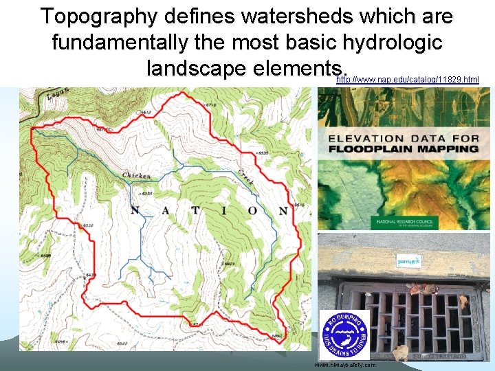
Topography defines watersheds which are fundamentally the most basic hydrologic landscape elements. http: //www. nap. edu/catalog/11829. html www. hiwaysafety. com

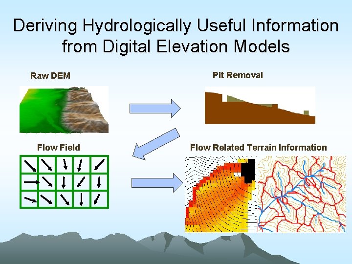
Deriving Hydrologically Useful Information from Digital Elevation Models Raw DEM Flow Field Pit Removal Flow Related Terrain Information

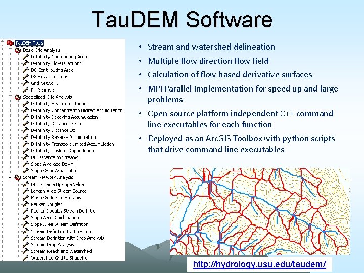
Tau. DEM Software • • Stream and watershed delineation Multiple flow direction flow field Calculation of flow based derivative surfaces MPI Parallel Implementation for speed up and large problems • Open source platform independent C++ command line executables for each function • Deployed as an Arc. GIS Toolbox with python scripts that drive command line executables http: //hydrology. usu. edu/taudem/

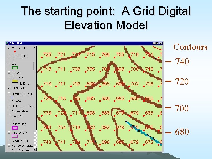
The starting point: A Grid Digital Elevation Model Contours 740 720 700 680

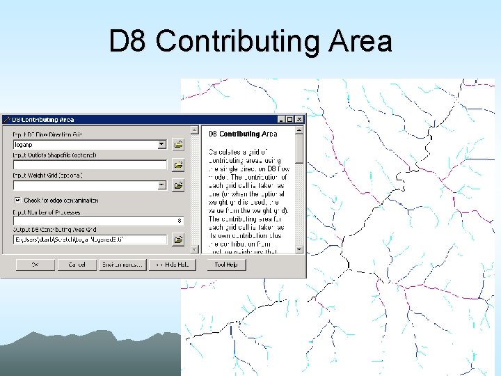
D 8 Contributing Area

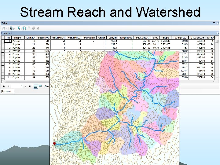
Stream Reach and Watershed

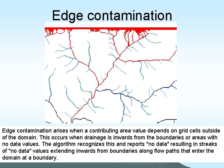
Edge contamination arises when a contributing area value depends on grid cells outside of the domain. This occurs when drainage is inwards from the boundaries or areas with no data values. The algorithm recognizes this and reports "no data" resulting in streaks of "no data" values extending inwards from boundaries along flow paths that enter the domain at a boundary.

Outline • Tau. DEM software • D-Infinity flow model • Generalized flow accumulation (Flow algebra) • Parallel algorithms • Programming

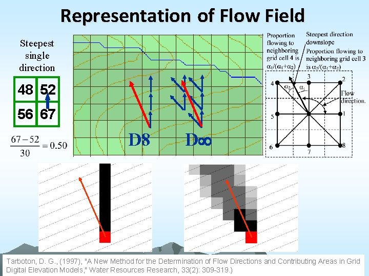
Representation of Flow Field Steepest single direction 48 52 56 67 D 8 D Tarboton, D. G. , (1997), "A New Method for the Determination of Flow Directions and Contributing Areas in Grid Digital Elevation Models, " Water Resources Research, 33(2): 309 -319. )

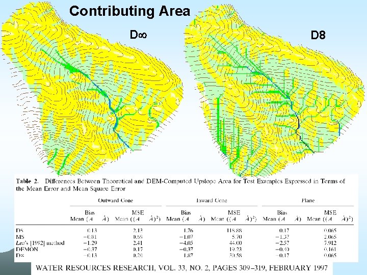
Contributing Area D D 8

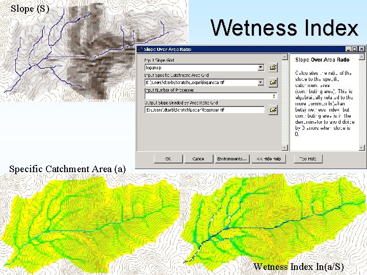
Slope (S) Wetness Index Specific Catchment Area (a) Wetness Index ln(a/S)

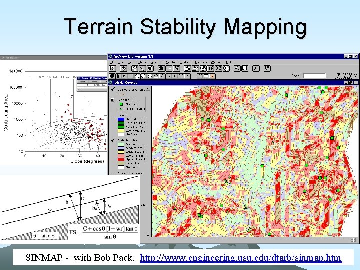
Terrain Stability Mapping SINMAP - with Bob Pack. http: //www. engineering. usu. edu/dtarb/sinmap. htm

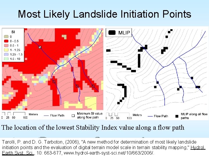
Most Likely Landslide Initiation Points The location of the lowest Stability Index value along a flow path Tarolli, P. and D. G. Tarboton, (2006), "A new method for determination of most likely landslide initiation points and the evaluation of digital terrain model scale in terrain stability mapping, " Hydrol. Earth Syst. Sci. , 10: 663 -677, www. hydrol-earth-syst-sci. net/10/663/2006/.

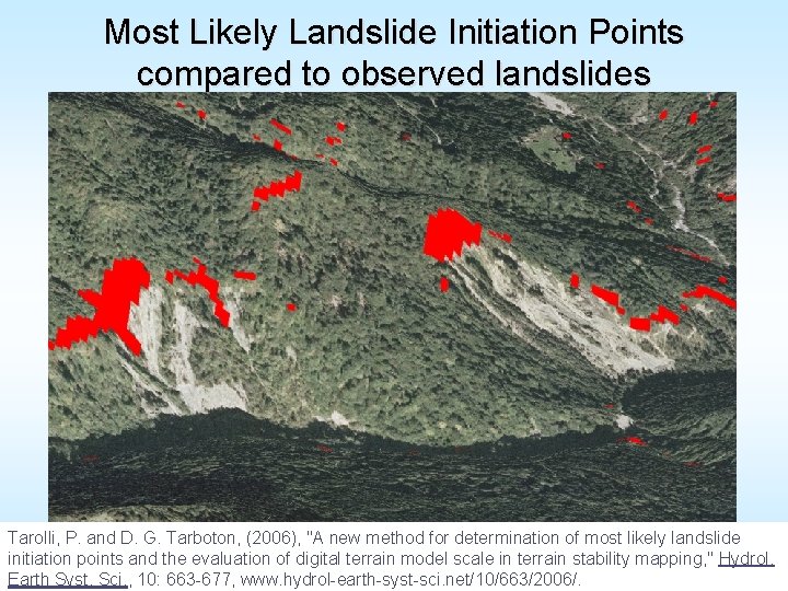
Most Likely Landslide Initiation Points compared to observed landslides Tarolli, P. and D. G. Tarboton, (2006), "A new method for determination of most likely landslide initiation points and the evaluation of digital terrain model scale in terrain stability mapping, " Hydrol. Earth Syst. Sci. , 10: 663 -677, www. hydrol-earth-syst-sci. net/10/663/2006/.

Outline • Tau. DEM software • D-Infinity flow model • Generalized flow accumulation (Flow algebra) • Parallel algorithms • Programming

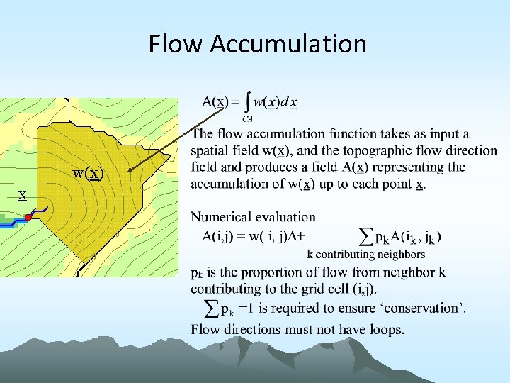
Flow Accumulation w(x) x

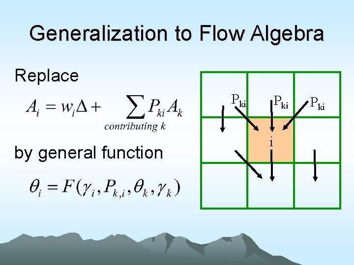
Generalization to Flow Algebra Replace Pki by general function Pki i Pki

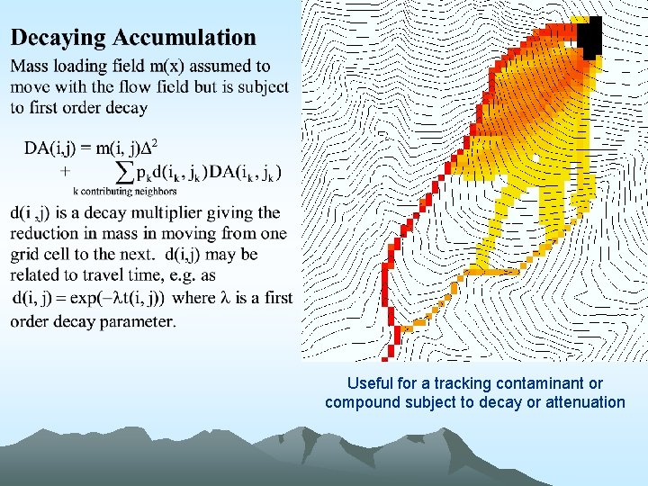
Useful for a tracking contaminant or compound subject to decay or attenuation

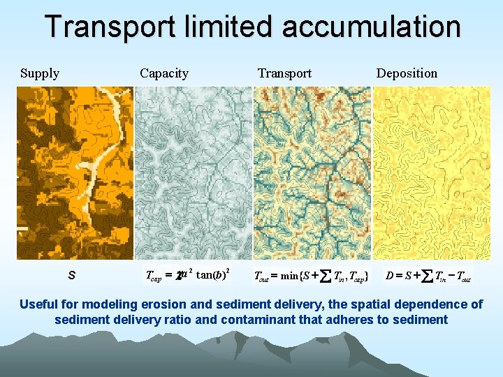
Transport limited accumulation Supply Capacity S Tcap = ca 2 tan(b) 2 Transport Tout = min{S + å Tin , Tcap} Deposition D = S + å Tin - Tout Useful for modeling erosion and sediment delivery, the spatial dependence of sediment delivery ratio and contaminant that adheres to sediment

Outline • Tau. DEM software • D-Infinity flow model • Generalized flow accumulation (Flow algebra) • Parallel algorithms • Programming

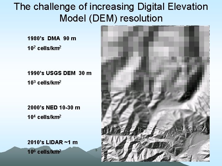
The challenge of increasing Digital Elevation Model (DEM) resolution 1980’s DMA 90 m 102 cells/km 2 1990’s USGS DEM 30 m 103 cells/km 2 2000’s NED 10 -30 m 104 cells/km 2 2010’s LIDAR ~1 m 106 cells/km 2

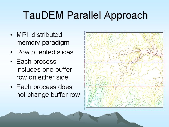
Tau. DEM Parallel Approach • MPI, distributed memory paradigm • Row oriented slices • Each process includes one buffer row on either side • Each process does not change buffer row

Tau. DEM Parallel Approach • MPI, distributed memory paradigm • Row oriented slices • Each process includes one buffer row on either side • Each process does not change buffer row

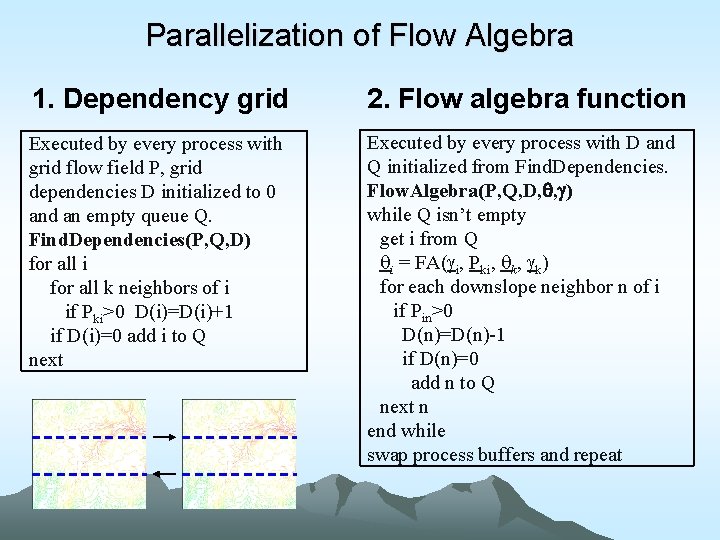
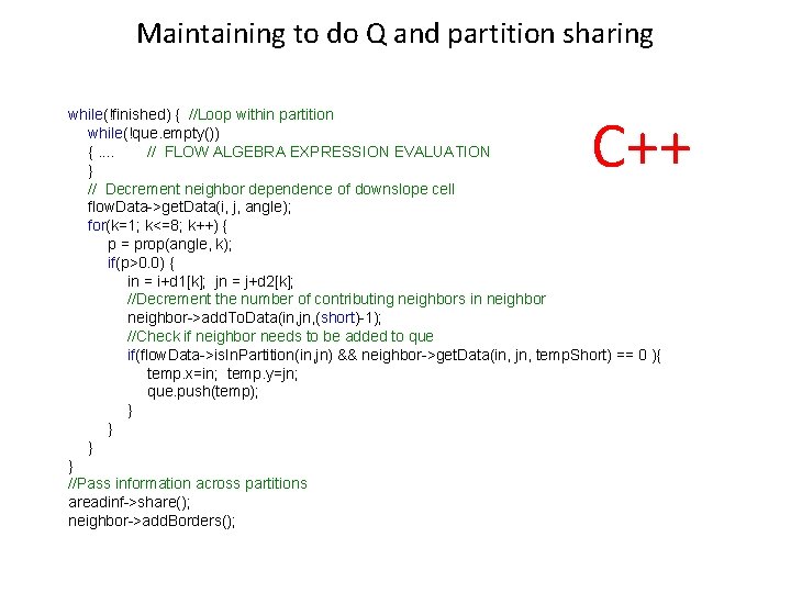
Parallelization of Flow Algebra 1. Dependency grid 2. Flow algebra function Executed by every process with grid flow field P, grid dependencies D initialized to 0 and an empty queue Q. Find. Dependencies(P, Q, D) for all i for all k neighbors of i if Pki>0 D(i)=D(i)+1 if D(i)=0 add i to Q next Executed by every process with D and Q initialized from Find. Dependencies. Flow. Algebra(P, Q, D, , ) while Q isn’t empty get i from Q i = FA( i, Pki, k) for each downslope neighbor n of i if Pin>0 D(n)=D(n)-1 if D(n)=0 add n to Q next n end while swap process buffers and repeat

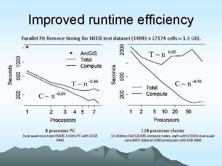
Improved runtime efficiency Parallel Pit Remove timing for NEDB test dataset (14849 x 27174 cells 1. 6 GB). 8 processor PC Dual quad-core Xeon E 5405 2. 0 GHz PC with 16 GB RAM 128 processor cluster 16 diskless Dell SC 1435 compute nodes, each with 2. 0 GHz dual quad -core AMD Opteron 2350 processors with 8 GB RAM

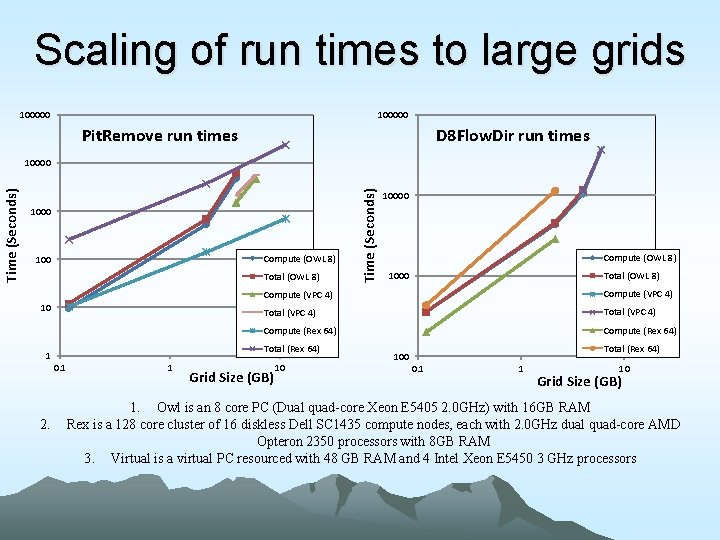
Scaling of run times to large grids 100000 Pit. Remove run times D 8 Flow. Dir run times 1000 Compute (OWL 8) 100 Total (OWL 8) 10 0. 1 2. 1 10000 Compute (OWL 8) 1000 Total (OWL 8) Compute (VPC 4) Total (VPC 4) Compute (Rex 64) Total (Rex 64) 1 Time (Seconds) 10000 Grid Size (GB) 10 Total (Rex 64) 100 0. 1 1 10 Grid Size (GB) 1. Owl is an 8 core PC (Dual quad-core Xeon E 5405 2. 0 GHz) with 16 GB RAM Rex is a 128 core cluster of 16 diskless Dell SC 1435 compute nodes, each with 2. 0 GHz dual quad-core AMD Opteron 2350 processors with 8 GB RAM 3. Virtual is a virtual PC resourced with 48 GB RAM and 4 Intel Xeon E 5450 3 GHz processors

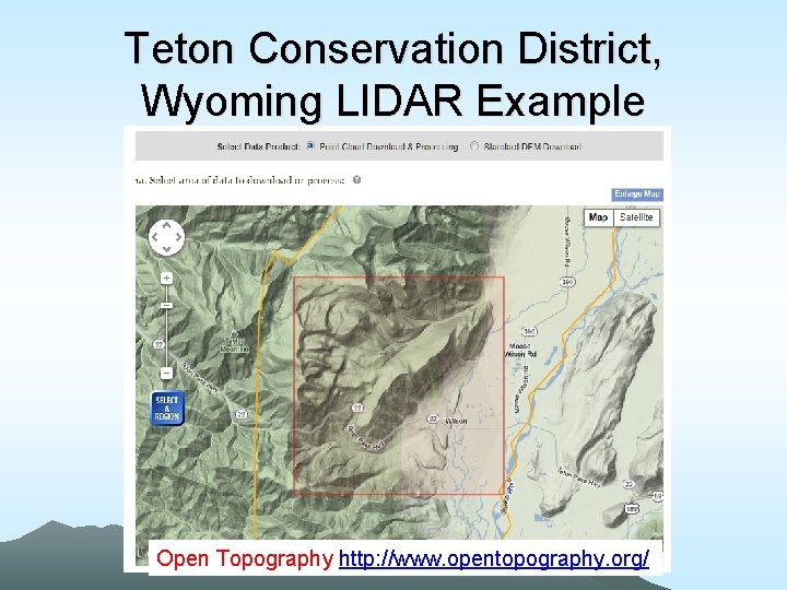
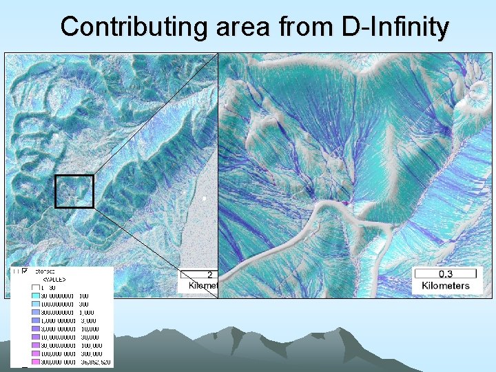
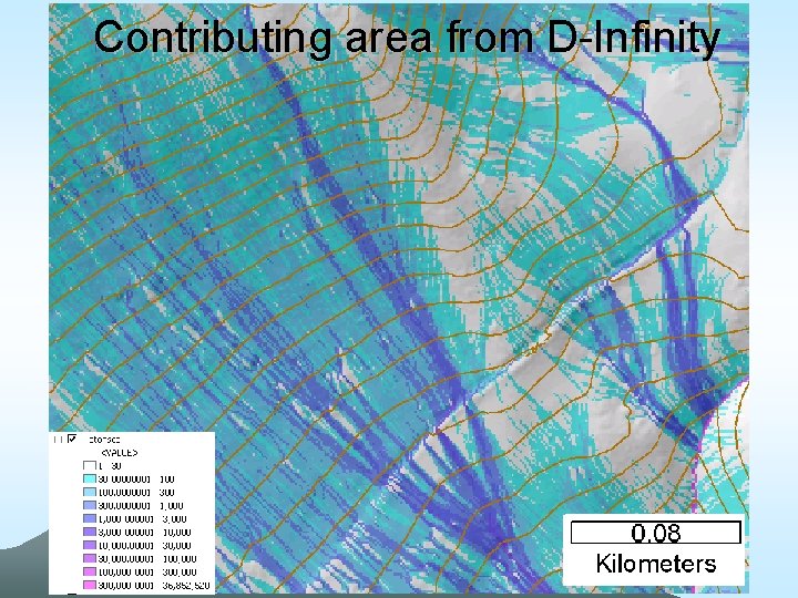
Teton Conservation District, Wyoming LIDAR Example Open Topography http: //www. opentopography. org/

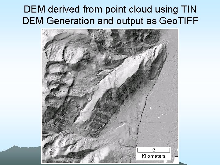
DEM derived from point cloud using TIN DEM Generation and output as Geo. TIFF

Contributing area from D-Infinity

Contributing area from D-Infinity

Outline • Tau. DEM software • D-Infinity flow model • Generalized flow accumulation (Flow algebra) • Parallel algorithms • Programming

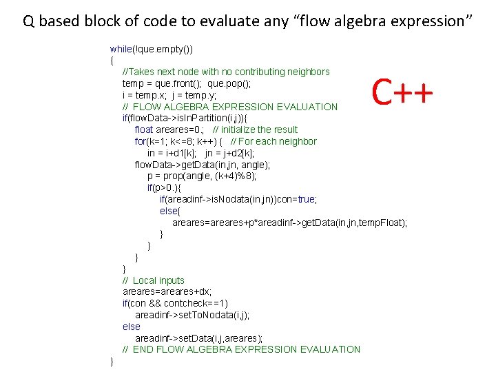
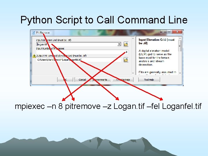
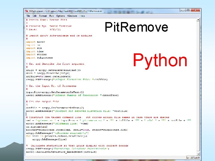
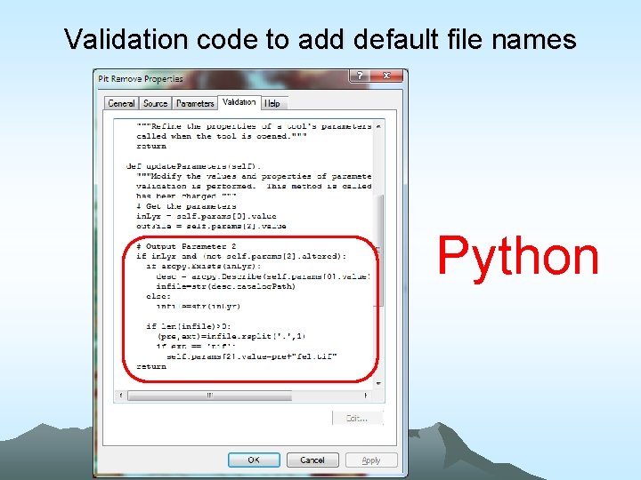
Programming • C++ Command Line Executables that use MPI • Arc. GIS Python Script Tools • Python validation code to provide file name defaults • Shared as Arc. GIS Toolbox

Q based block of code to evaluate any “flow algebra expression” while(!que. empty()) { //Takes next node with no contributing neighbors temp = que. front(); que. pop(); i = temp. x; j = temp. y; // FLOW ALGEBRA EXPRESSION EVALUATION if(flow. Data->is. In. Partition(i, j)){ float areares=0. ; // initialize the result for(k=1; k<=8; k++) { // For each neighbor in = i+d 1[k]; jn = j+d 2[k]; flow. Data->get. Data(in, jn, angle); p = prop(angle, (k+4)%8); if(p>0. ){ if(areadinf->is. Nodata(in, jn))con=true; else{ areares=areares+p*areadinf->get. Data(in, jn, temp. Float); } } // Local inputs areares=areares+dx; if(con && contcheck==1) areadinf->set. To. Nodata(i, j); else areadinf->set. Data(i, j, areares); // END FLOW ALGEBRA EXPRESSION EVALUATION } C++

Maintaining to do Q and partition sharing C++ while(!finished) { //Loop within partition while(!que. empty()) {. . // FLOW ALGEBRA EXPRESSION EVALUATION } // Decrement neighbor dependence of downslope cell flow. Data->get. Data(i, j, angle); for(k=1; k<=8; k++) { p = prop(angle, k); if(p>0. 0) { in = i+d 1[k]; jn = j+d 2[k]; //Decrement the number of contributing neighbors in neighbor->add. To. Data(in, jn, (short)-1); //Check if neighbor needs to be added to que if(flow. Data->is. In. Partition(in, jn) && neighbor->get. Data(in, jn, temp. Short) == 0 ){ temp. x=in; temp. y=jn; que. push(temp); } } //Pass information across partitions areadinf->share(); neighbor->add. Borders();

Python Script to Call Command Line mpiexec –n 8 pitremove –z Logan. tif –fel Loganfel. tif

Pit. Remove Python

Validation code to add default file names Python

Some Tau. DEM Demo’s • And fixing one of the functions …

Conclusions Ø The GIS grid based terrain flow data model enables derivation of a wide variety of information useful for the study of hydrologic processes. Ø Terrain surface derivatives enhanced by use of DInfinity model. Ø Flow algebra a general “recipe” for terrain flow related modeling. Ø Parallelism required to process big terrain data. Ø Saw how to dip into GIS based programming