1 Structural Equation Modeling for Ecologists Using R

1 Structural Equation Modeling for Ecologists Using R JOHN KITCHENER SAKALUK UNIVERSITY OF VICTORIA DEPARTMENT OF PSYCHOLOGY https: //osf. io/zn 3 fg/

2 About These Workshop Materials

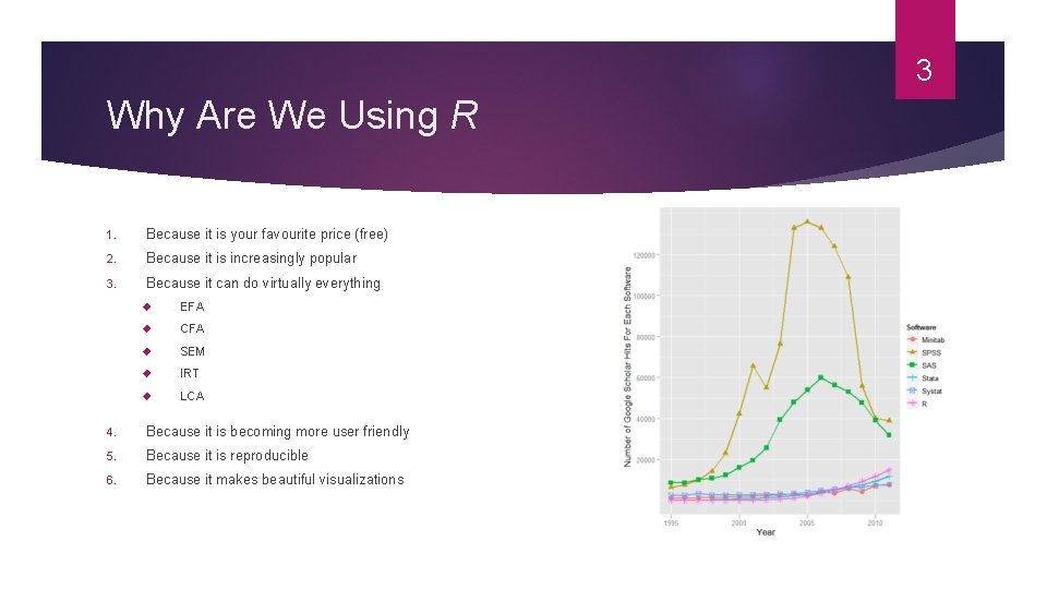
3 Why Are We Using R 1. Because it is your favourite price (free) 2. Because it is increasingly popular 3. Because it can do virtually everything EFA CFA SEM IRT LCA 4. Because it is becoming more user friendly 5. Because it is reproducible 6. Because it makes beautiful visualizations

4 Today’s Agenda 1. Orienting you to R (importing data, using packages) 2. Why SEM, as an Ecologist? 3. Fundamentals of CFA 4. Advanced CFA 5. SEM and Multi-Group SEM

5 An Orientation to R/R-Studio

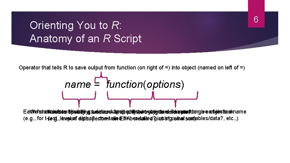
Orienting You to R: Anatomy of an R Script Operator that tells R to save output from function (on right of =) into object (named on left of =) name = function(options) Each function has flexibility; we need to specify how we want it to perform a certain task We store information (e. g. , data, output, plots) in objects—we need to give objects a name Need to specify a function--what are we trying to do/create? (e. g. , for t-test, level of alpha? , one-tailed or two-tailed? , using what variables/data? , etc. , ) (e. g. , import data, perform an EFA, create a plot of some sort) 6

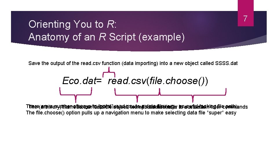
Orienting You to R: Anatomy of an R Script (example) 7 Save the output of the read. csv function (data importing) into a new object called SSSS. dat Eco. dat= read. csv(file. choose()) There a number of ways to “point” read. csv to a data file (e. g. , an awful-looking file path). The (arbitrary) name for our data file object; we will use it to refer to our data in later commands The read. csv function is used to import data that is in a. csv file The file. choose() option pulls up a navigation menu to make selecting data file *super* easy

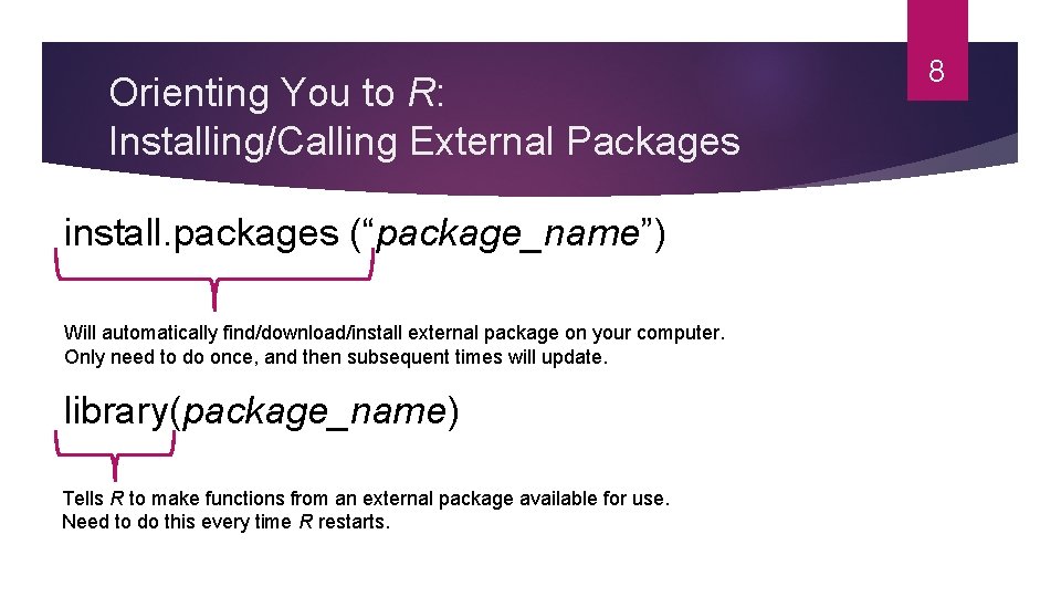
Orienting You to R: Installing/Calling External Packages install. packages (“package_name”) Will automatically find/download/install external package on your computer. Only need to do once, and then subsequent times will update. library(package_name) Tells R to make functions from an external package available for use. Need to do this every time R restarts. 8

9 Check Out Section (1) of Script 1. See how comments/headings in R help to organize your code 2. Learn how to install/call packages, and request citation info to give developers credit 3. Import example data OR your own data

10 Why Use SEM?

11 Why Consider Using SEM? 1. Multiple outcome variables 2. Modeling (vs. making) assumptions 3. Model comparison/constraint testing 4. Latent variables*

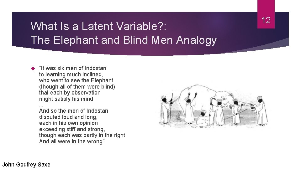
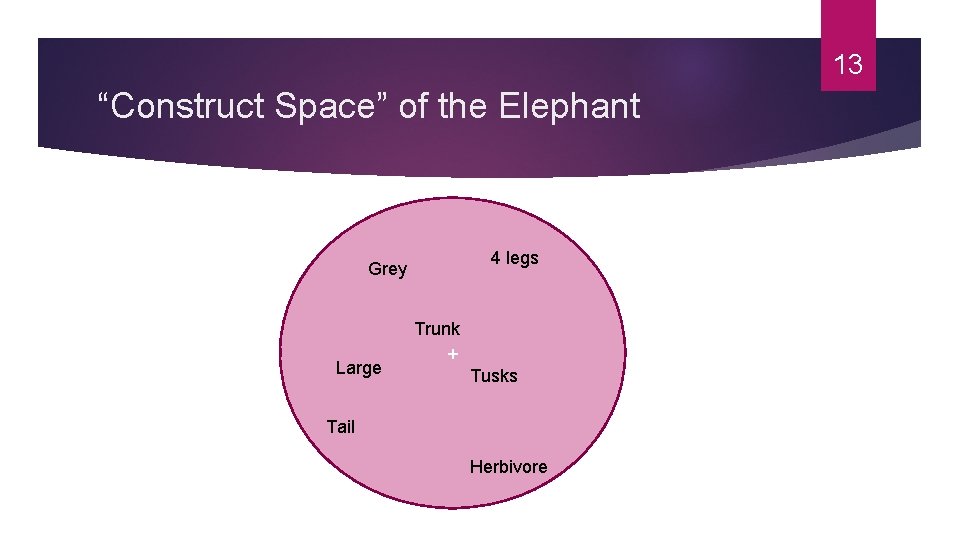
What Is a Latent Variable? : The Elephant and Blind Men Analogy “It was six men of Indostan to learning much inclined, who went to see the Elephant (though all of them were blind) that each by observation might satisfy his mind … And so the men of Indostan disputed loud and long, each in his own opinion exceeding stiff and strong, though each was partly in the right And all were in the wrong” John Godfrey Saxe 12

13 “Construct Space” of the Elephant 4 legs Grey Large Trunk + Tusks Tail Herbivore

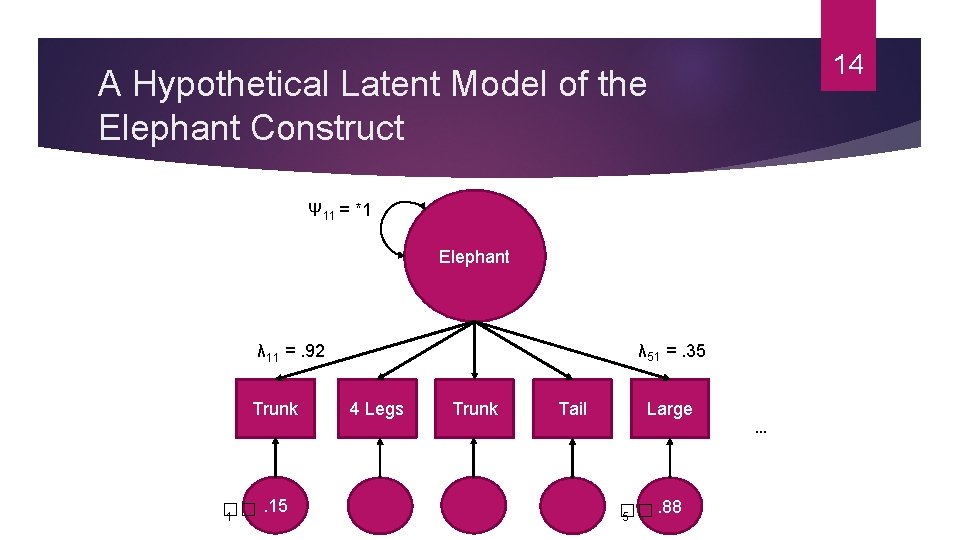
14 A Hypothetical Latent Model of the Elephant Construct Ψ 11 = *1 Elephant λ 51 =. 35 λ 11 =. 92 Trunk . 15 �� 1 4 Legs Trunk Tail Large . 88 �� 5 …

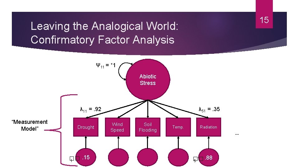
15 Leaving the Analogical World: Confirmatory Factor Analysis Ψ 11 = *1 Abiotic Stress λ 51 =. 35 λ 11 =. 92 “Measurement Model” Drought . 15 �� 1 Wind Speed Soil Flooding Temp. Radiation . 88 �� 5 …

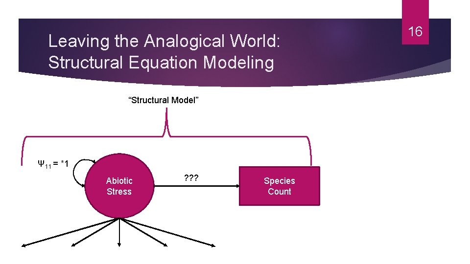
Leaving the Analogical World: Structural Equation Modeling “Structural Model” Ψ 11 = *1 Abiotic Stress ? ? ? Species Count 16

17 Leaving the Analogical World: Structural Equation Modeling Ψ 11 = *1 Abiotic Stress ? ? ? Ψ 22 = *1 Biodiversity

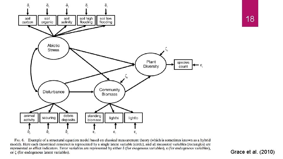
18 Grace et al. (2010)

Considerations for Ecologists Modeling Latent Variables (LVs) Requires multiple indicators of the LVs I. e. , Collection of data from more observed variables Why bother? Theoretical precision Increased statistical power for inferential tests of structural parameters How do LVs facilitate this? 19

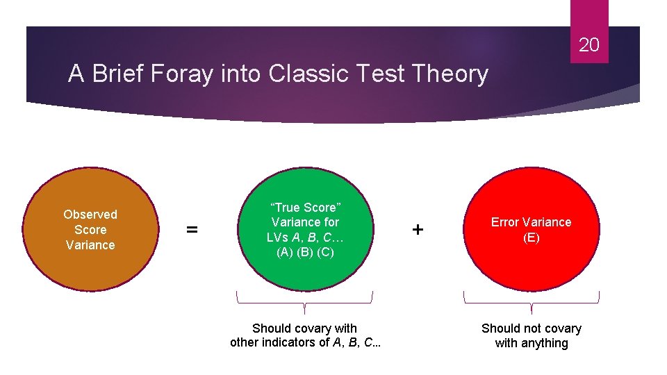
20 A Brief Foray into Classic Test Theory Observed Score Variance = “True Score” Variance for LVs A, B, C… (A) (B) (C) Should covary with other indicators of A, B, C… + Error Variance (E) Should not covary with anything

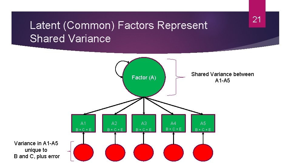
Latent (Common) Factors Represent Shared Variance between A 1 -A 5 Factor (A) Variance in A 1 -A 5 unique to B and C, plus error 21 A 2 A 3 A 4 A 5 B + C + E B + C + E

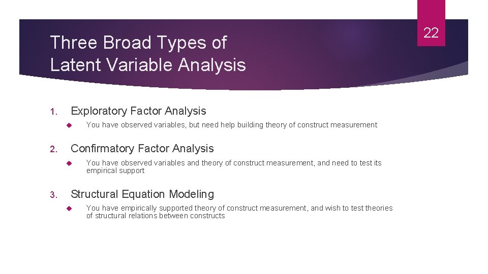
Three Broad Types of Latent Variable Analysis 1. Exploratory Factor Analysis 2. Confirmatory Factor Analysis 3. You have observed variables, but need help building theory of construct measurement You have observed variables and theory of construct measurement, and need to test its empirical support Structural Equation Modeling You have empirically supported theory of construct measurement, and wish to test theories of structural relations between constructs 22

23 “All models are wrong, but some are useful” --George Box (1978), Statistician

24 CFA Basic Principles

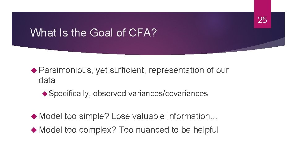
25 What Is the Goal of CFA? Parsimonious, yet sufficient, representation of our data Specifically, observed variances/covariances Model too simple? Lose valuable information… Model too complex? Too nuanced to be helpful

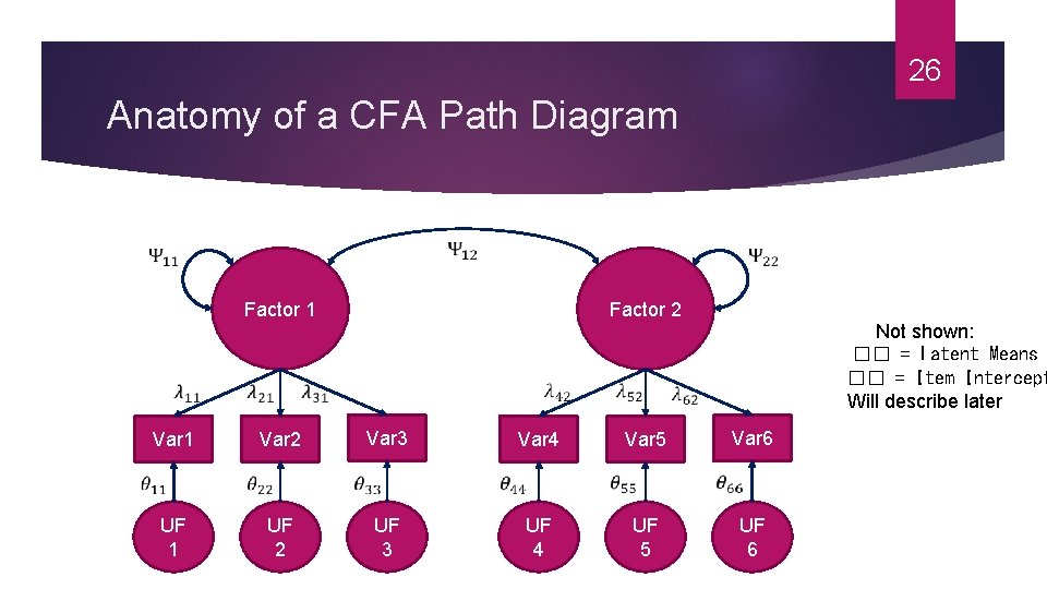
26 Anatomy of a CFA Path Diagram Factor 1 UF 1 Var 3 UF 2 Var 2 Var 1 Factor 2 Var 4 UF 3 UF 4 Var 6 Var 5 Not shown: �� = Latent Means �� = Item Intercept Will describe later UF 5 UF 6

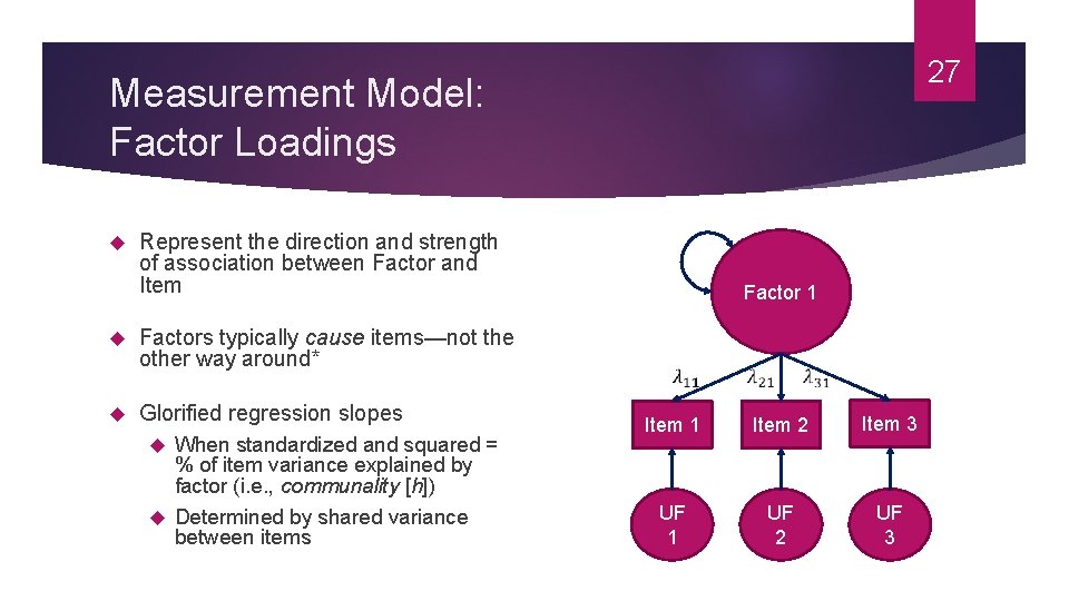
27 Measurement Model: Factor Loadings Represent the direction and strength of association between Factor and Item Factors typically cause items—not the other way around* Glorified regression slopes When standardized and squared = % of item variance explained by factor (i. e. , communality [h]) Determined by shared variance between items Factor 1 Item 1 Item 2 Item 3 UF 1 UF 2 UF 3

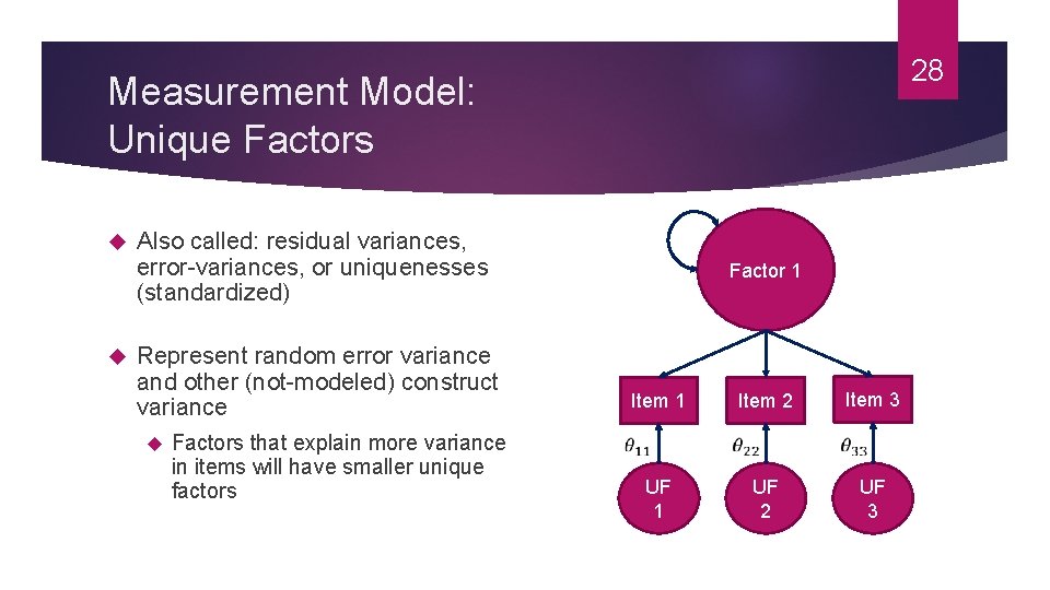
28 Measurement Model: Unique Factors Also called: residual variances, error-variances, or uniquenesses (standardized) Represent random error variance and other (not-modeled) construct variance Factors that explain more variance in items will have smaller unique factors Factor 1 Item 2 Item 3 UF 1 UF 2 UF 3

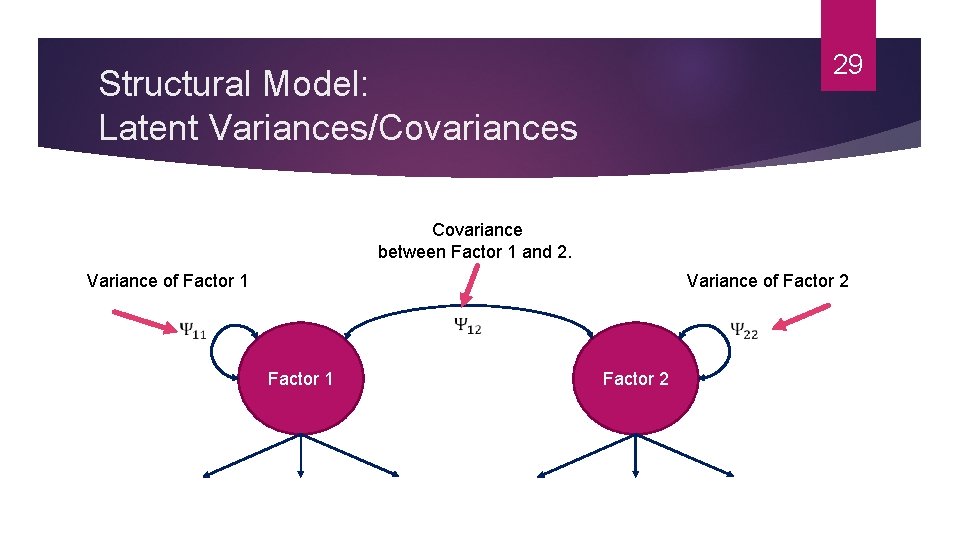
29 Structural Model: Latent Variances/Covariances Covariance between Factor 1 and 2. Variance of Factor 1 Variance of Factor 2 Factor 1 Factor 2

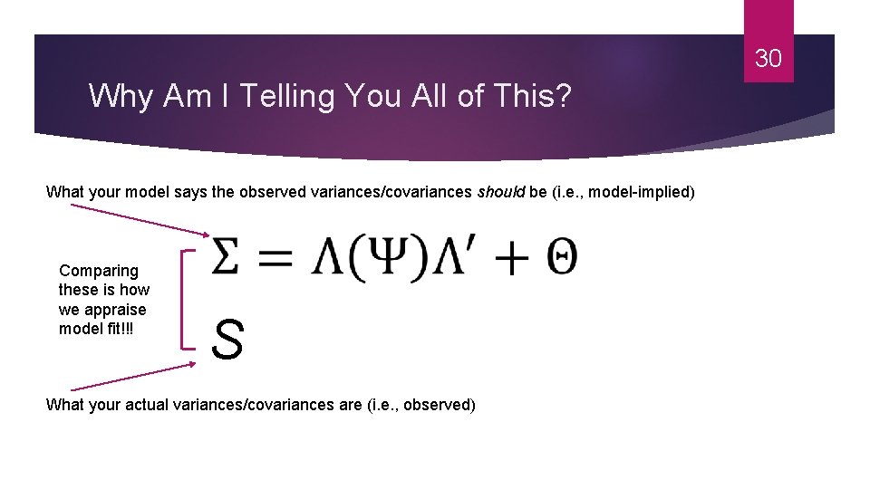
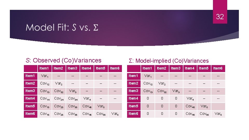
30 Why Am I Telling You All of This? What your model says the observed variances/covariances should be (i. e. , model-implied) Comparing these is how we appraise model fit!!! S What your actual variances/covariances are (i. e. , observed)

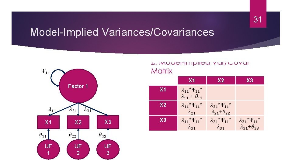
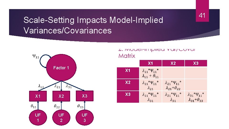
31 Model-Implied Variances/Covariances X 1 Factor 1 UF 1 X 2 X 3 X 2 X 1 UF 2 UF 3 X 2 X 3

32 S: Observed (Co)Variances Σ: Model-implied (Co)Variances Item 1 Item 2 Item 3 Item 4 Item 5 Item 6 Item 1 Var 1 -- -- -- Item 2 Cov 12 Var 2 -- -- Item 3 Cov 13 Cov 32 Var 3 -- -- -- Item 4 Cov 14 Cov 24 Cov 34 Var 4 -- -- Item 4 0 0 0 Var 4 -- -- Item 5 Cov 15 Cov 25 Cov 35 Cov 45 Var 5 Item 5 0 0 0 Cov 45 Var 5 Item 6 Cov 16 Cov 26 Cov 36 Cov 46 Cov 56 Item 6 0 0 0 Cov 46 Cov 56 Var 6

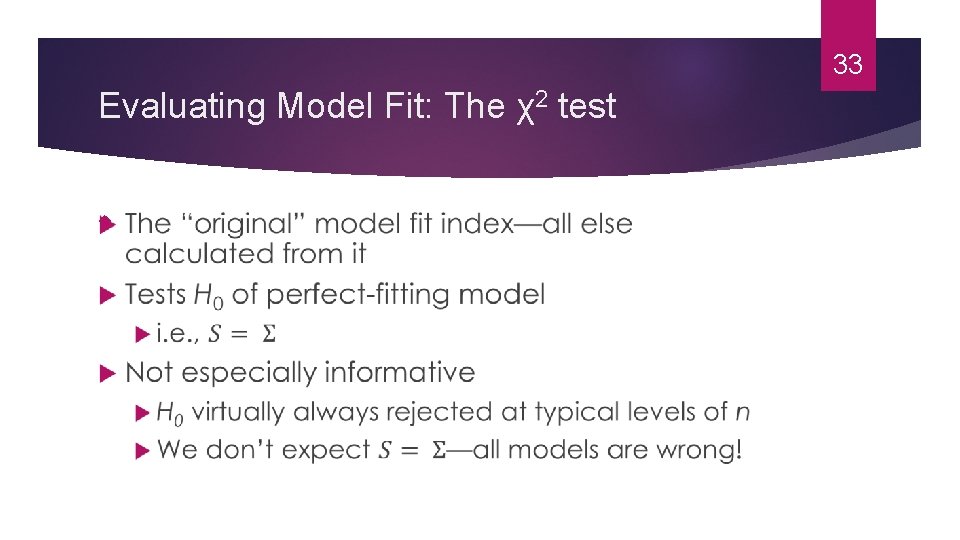
33 Evaluating Model Fit: The χ2 test

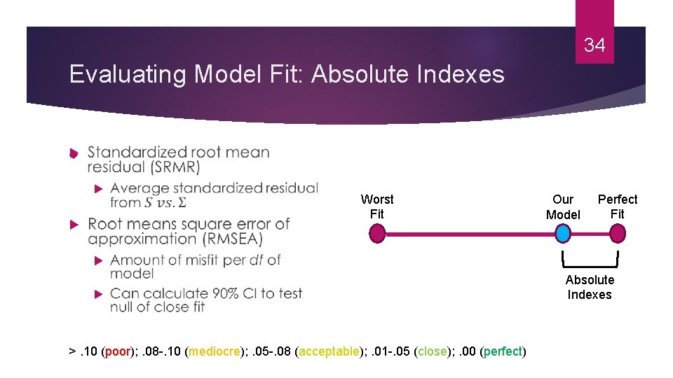
34 Evaluating Model Fit: Absolute Indexes Worst Fit Our Model Perfect Fit Absolute Indexes >. 10 (poor); . 08 -. 10 (mediocre); . 05 -. 08 (acceptable); . 01 -. 05 (close); . 00 (perfect)

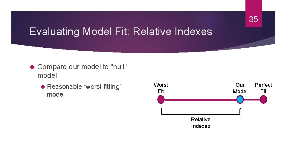
35 Evaluating Model Fit: Relative Indexes Compare our model to “null” model Reasonable “worst-fitting” model Worst Fit Our Model Relative Indexes Perfect Fit

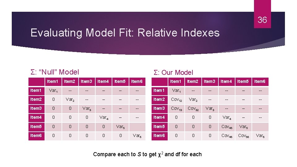
36 Evaluating Model Fit: Relative Indexes Σ: “Null” Model Σ: Our Model Item 1 Item 2 Item 3 Item 4 Item 5 Item 6 Item 1 Var 1 -- -- -- Item 2 0 Var 2 -- -- Item 2 Cov 12 Var 2 -- -- Item 3 0 0 Var 3 -- -- -- Item 3 Cov 13 Cov 32 Var 3 -- -- -- Item 4 0 0 0 Var 4 -- -- Item 5 0 0 Var 5 Item 5 0 0 0 Cov 45 Var 5 Item 6 0 0 0 Cov 46 Cov 56 Var 6 Compare each to S to get χ2 and df for each Var 6

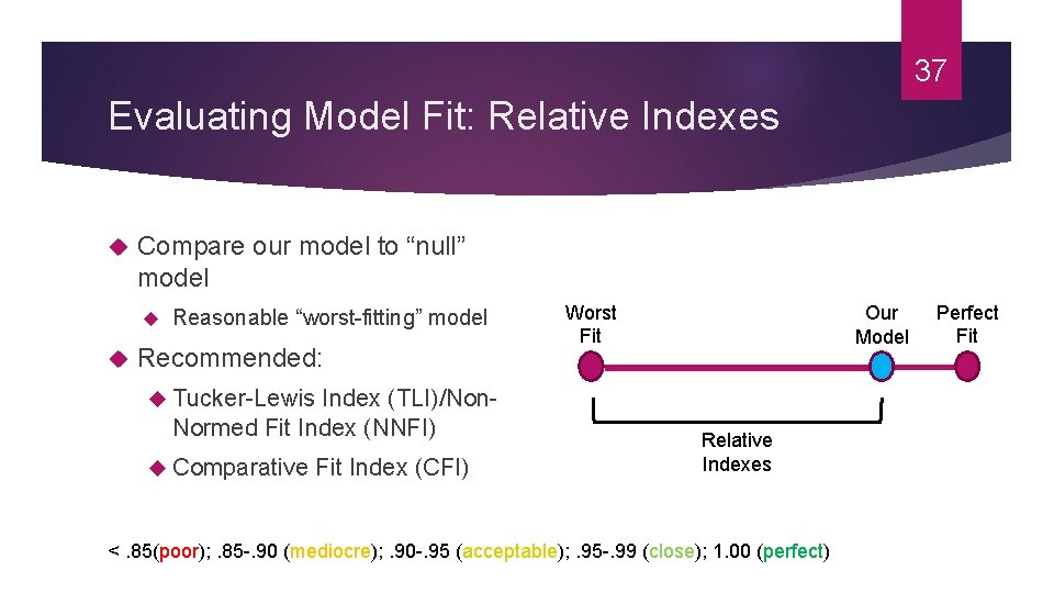
37 Evaluating Model Fit: Relative Indexes Compare our model to “null” model Reasonable “worst-fitting” model Recommended: Worst Fit Our Model Tucker-Lewis Index (TLI)/Non- Normed Fit Index (NNFI) Comparative Fit Index (CFI) Relative Indexes <. 85(poor); . 85 -. 90 (mediocre); . 90 -. 95 (acceptable); . 95 -. 99 (close); 1. 00 (perfect) Perfect Fit

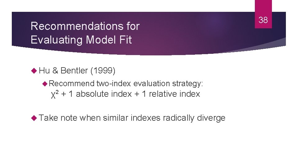
Recommendations for Evaluating Model Fit Hu & Bentler (1999) Recommend two-index evaluation strategy: χ2 + 1 absolute index + 1 relative index Take note when similar indexes radically diverge 38

39 But There’s A Problem or Two… 1. Scale-setting: Latent variables are “unobservable”– how do we come to understand their scale? We need a reference point of some kind. 2. Identification: Many unknowns to solve for. We need to ensure the equations for the model are solvable.

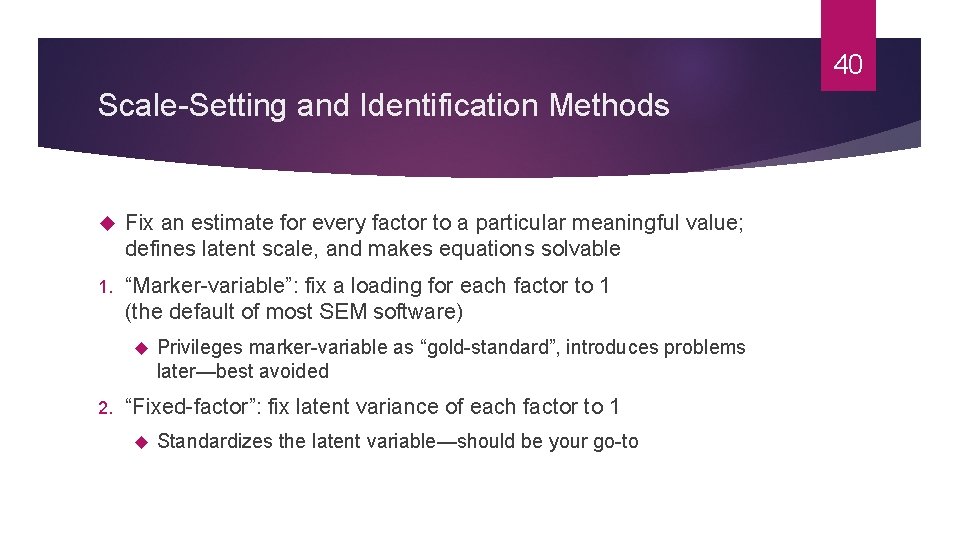
40 Scale-Setting and Identification Methods Fix an estimate for every factor to a particular meaningful value; defines latent scale, and makes equations solvable 1. “Marker-variable”: fix a loading for each factor to 1 (the default of most SEM software) 2. Privileges marker-variable as “gold-standard”, introduces problems later—best avoided “Fixed-factor”: fix latent variance of each factor to 1 Standardizes the latent variable—should be your go-to

41 Scale-Setting Impacts Model-Implied Variances/Covariances X 1 Factor 1 UF 1 X 2 X 3 X 2 X 1 UF 2 UF 3 X 2 X 3

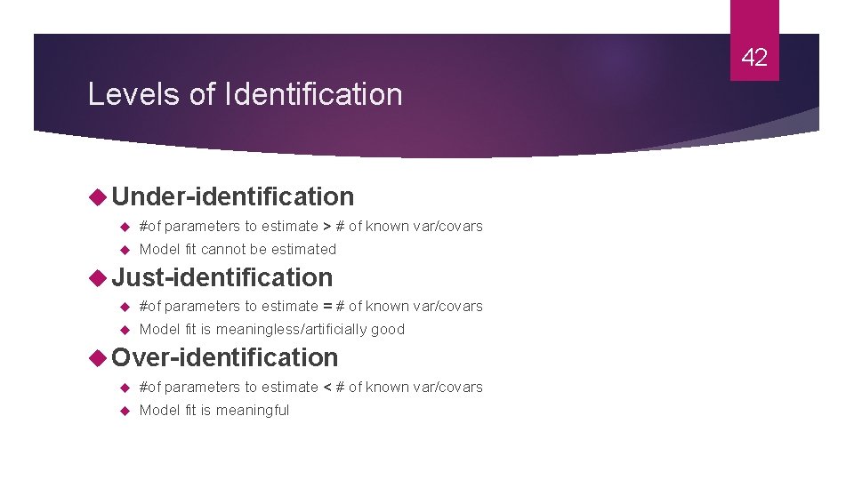
42 Levels of Identification Under-identification #of parameters to estimate > # of known var/covars Model fit cannot be estimated Just-identification #of parameters to estimate = # of known var/covars Model fit is meaningless/artificially good Over-identification #of parameters to estimate < # of known var/covars Model fit is meaningful

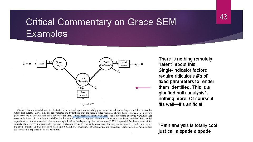
Critical Commentary on Grace SEM Examples There is nothing remotely “latent” about this. Single-indicator factors require ridiculous #’s of fixed parameters to render them identified. This is a glorified path-analysis*, nothing more. Of course it fits well—it’s artificial! *Path analysis is totally cool; just call a spade 43

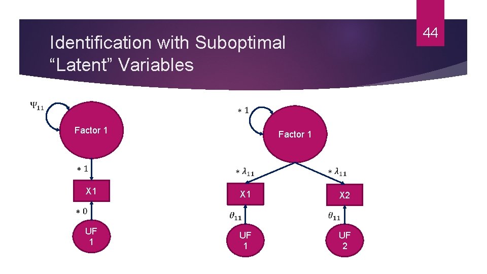
44 Identification with Suboptimal “Latent” Variables Factor 1 X 1 X 2 UF 1 UF 2

45 CFA in lavaan() (Section (2) of Script) 1. Save CFA model syntax in an R object 2. Fit CFA model and specify scale-setting method; save output in a new object 3. Request summary output from CFA object

46 Advanced CFA

If Your CFA Model Fit Is Unacceptably Bad… Tread carefully! Any model revisions are now exploratory You will be tempted to justify *anything* for good fit Replication is a must Software will produce “mod indexes” on request What model changes in current sample would improve model fit the most 47

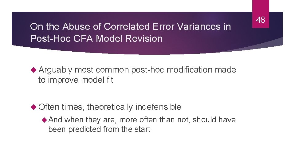
On the Abuse of Correlated Error Variances in Post-Hoc CFA Model Revision Arguably most common post-hoc modification made to improve model fit Often times, theoretically indefensible And when they are, more often than not, should have been predicted from the start 48

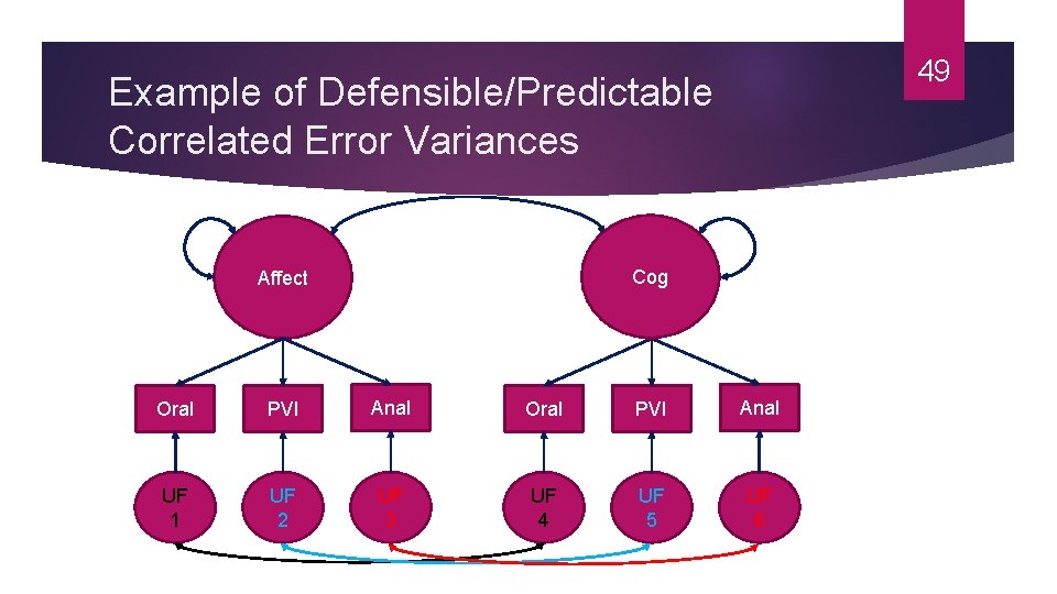
49 Example of Defensible/Predictable Correlated Error Variances Cog Affect Oral PVI Anal UF 1 UF 2 UF 3 UF 4 UF 5 UF 6

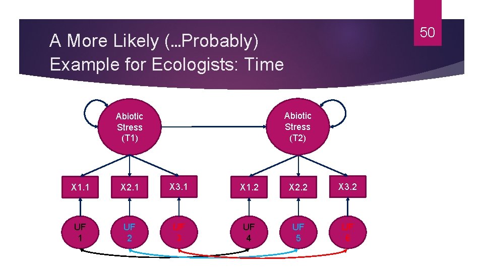
50 A More Likely (…Probably) Example for Ecologists: Time Abiotic Stress (T 2) Abiotic Stress (T 1) X 1. 1 X 2. 1 X 3. 1 X 1. 2 X 2. 2 X 3. 2 UF 1 UF 2 UF 3 UF 4 UF 5 UF 6

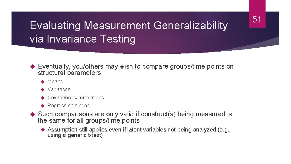
Evaluating Measurement Generalizability via Invariance Testing Eventually, you/others may wish to compare groups/time points on structural parameters Means Variances Covariances/correlations Regression slopes Such comparisons are only valid if construct(s) being measured is the same for all groups/time points Assumption still applies even if latent variables not being analyzed (e. g. , using a generic t-test) 51

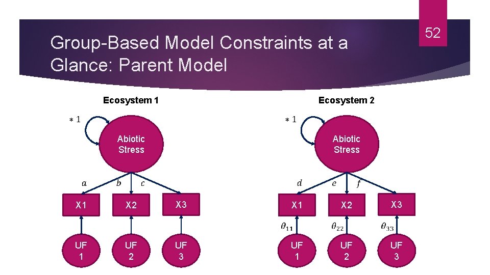
52 Group-Based Model Constraints at a Glance: Parent Model Ecosystem 2 Ecosystem 1 Abiotic Stress X 1 X 2 X 3 UF 2 UF 3 UF 1 X 3 X 2 X 1 UF 2 UF 3

53 Group-Based Model Constraints at a Glance: Nested Model Ecosystem 2 Ecosystem 1 Abiotic Stress X 1 X 2 X 3 UF 2 UF 3 UF 1 X 3 X 2 X 1 UF 2 UF 3

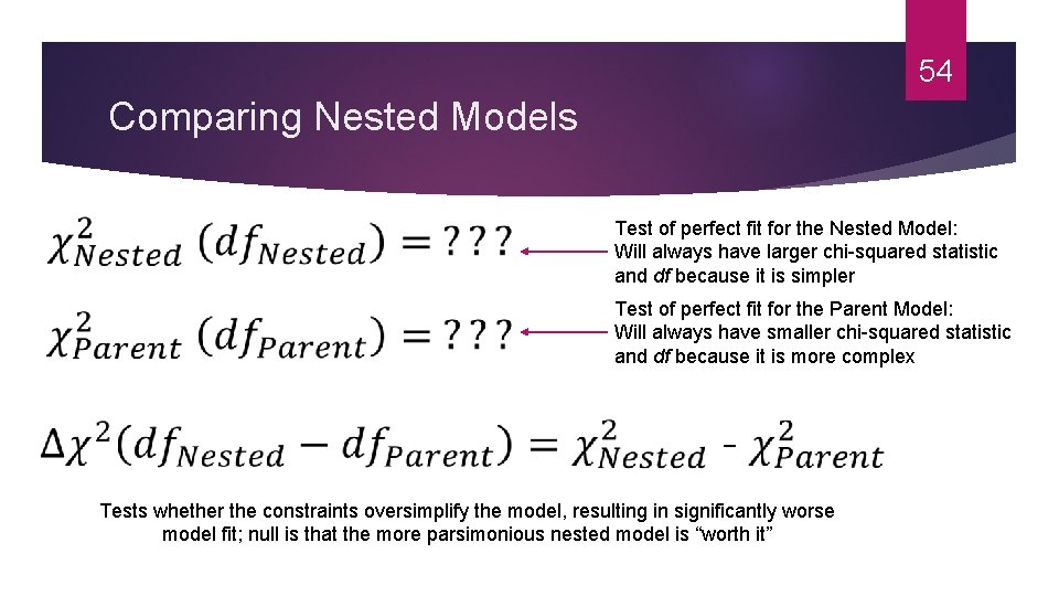
54 Comparing Nested Models Test of perfect fit for the Nested Model: Will always have larger chi-squared statistic and df because it is simpler Test of perfect fit for the Parent Model: Will always have smaller chi-squared statistic and df because it is more complex Tests whether the constraints oversimplify the model, resulting in significantly worse model fit; null is that the more parsimonious nested model is “worth it”

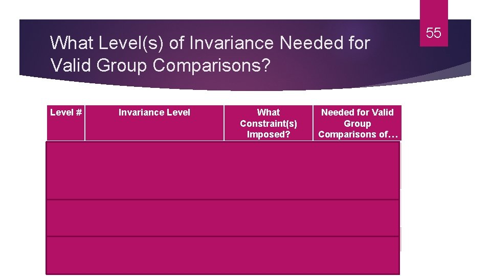
What Level(s) of Invariance Needed for Valid Group Comparisons? Level # Invariance Level What Constraint(s) Imposed? Needed for Valid Group Comparisons of… 1 “Configural”/“Pattern” Same # of factors, All structural and same pattern of parameters items loading onto factors 2 “Weak”/ “Loading”/ “Metric” 1 + equivalent factor loadings Variances, covariances, and regression slopes 3 “Strong”/“Intercept” 1 + 2 + equivalent intercepts Means 55

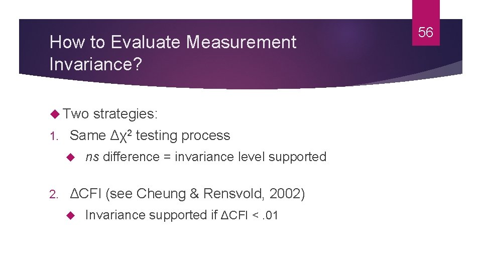
How to Evaluate Measurement Invariance? Two strategies: 1. Same Δχ2 testing process 2. ns difference = invariance level supported ΔCFI (see Cheung & Rensvold, 2002) Invariance supported if ΔCFI <. 01 56

In-Depth Theory Testing via CFA in R (section (3) in code) Request mod indexes for CFA model Use sem. Tools() package for easy testing of measurement invariance 57

58 Structural Equation Modeling

59 From CFA to SEM Analytic focus on structural level of the model Latent means, correlations, specifying regression pathways, etc. , Major perk of SEM w/ latent variables: more statistical power Bigger effects or less variability, depending on scale-setting

60 Traditional SEM: Fancy Multiple Regression Models Light Abiotic Stress a Biodiversity b Disturbance

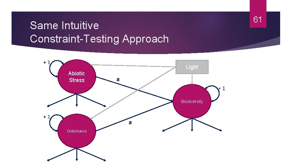
61 Same Intuitive Constraint-Testing Approach Light Abiotic Stress a Biodiversity a Disturbance

Group Comparisons of Latent Means (e. g. , latent t-test or ANOVA) sem. Tools() measurement. Invariance() command tests this by default Constrains all means to equality (omnibus test) Nested in strong/intercept invariance model Requires follow-up tests, if more than 2 groups 62

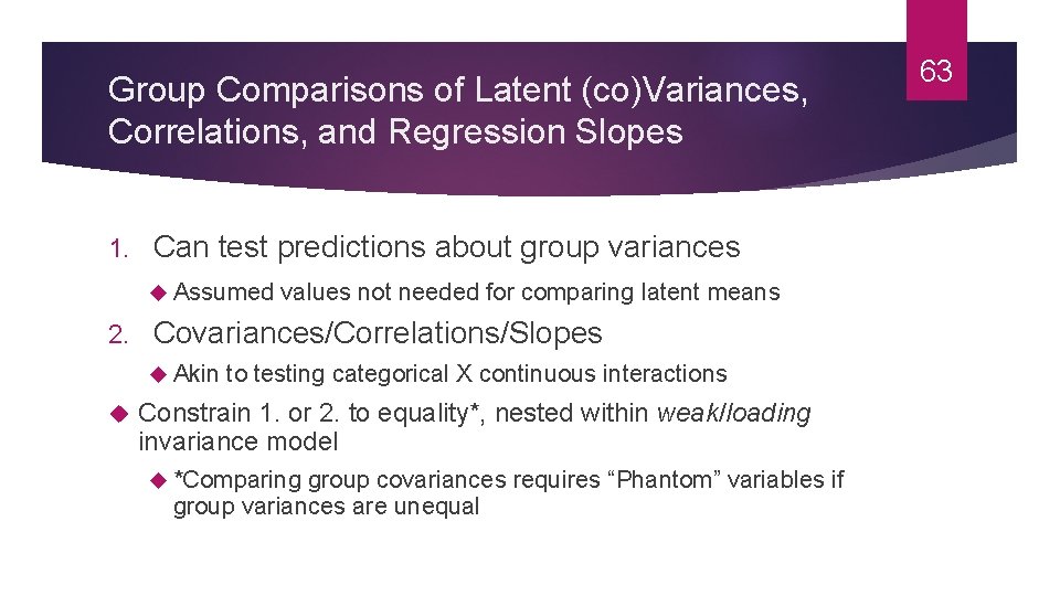
Group Comparisons of Latent (co)Variances, Correlations, and Regression Slopes 1. Can test predictions about group variances Assumed values not needed for comparing latent means 2. Covariances/Correlations/Slopes Akin to testing categorical X continuous interactions Constrain 1. or 2. to equality*, nested within weak/loading invariance model *Comparing group covariances requires “Phantom” variables if group variances are unequal 63

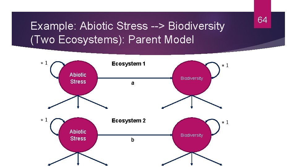
Example: Abiotic Stress --> Biodiversity (Two Ecosystems): Parent Model Ecosystem 1 Abiotic Stress a Biodiversity Ecosystem 2 Abiotic Stress b Biodiversity 64

Example: Abiotic Stress --> Biodiversity (Two Ecosystems): Nested Model Ecosystem 1 Abiotic Stress a Biodiversity Ecosystem 2 Abiotic Stress a Biodiversity 65

66 SEM Considerations Scale-setting method matters #1 reason marker-variable sucks: biases results of significance testing of structural estimates involving the latent variable; USE FIXEDFACTOR! Model complexity matters (especially with small samples) Convergence/estimation problems common when too much is asked of smaller amounts of data

67 Structural Equation Modeling via R 1. Fit measurement model for all variables to-be analyzed 2. Specify latent regressions and test for constraint of equal predictive strength 3. Specify multiple group latent regressions and test for constraint of equal predictive strength between groups

68 Resources for You See selected list of references for latent variable analysis Most informed this talk Stack. Exchange and Cross. Validated Online Q&A communities for programming and stats Psych. MAP and Psychological Methods Discussion FB Groups Twitter

69 Thank You! AND GOOD LUCK!