1 Status on realtime optimization as seen both

1 Status on real-time optimization as seen both from an industrial and academic point of view Elvira Marie B. Aske Department of Chemical Engineering Trondheim, March 27, 2009 Elvira Marie B. Aske, Trial lecture

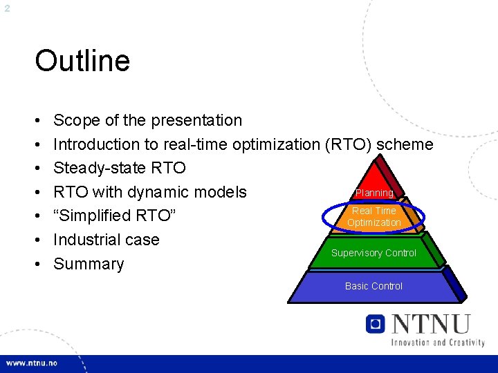
2 Outline • • Scope of the presentation Introduction to real-time optimization (RTO) scheme Steady-state RTO Planning RTO with dynamic models Real Time “Simplified RTO” Optimization Industrial case Supervisory Control Summary Basic Control

3 What is meant by real-time optimization? Definition [Engell, 2007]: ”a model based, upperlevel control system that is operated in closed loop and provides set-points to the lower-level control systems in order to maintain the process operation as close as possible to the economic optimum” The interpretations of RTO are many

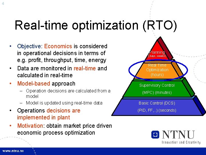
4 Real-time optimization (RTO) • Objective: Economics is considered in operational decisions in terms of e. g. profit, throughput, time, energy • Data are monitored in real-time and calculated in real-time • Model-based approach – Operation decisions are calculated from a model – Model is updated using real-time data • Operations decisions are implemented in plant • Motivation: obtain market price driven economic process optimization Planning (days, weeks) Real Time Optimization (hours) Supervisory Control (MPC) (minutes) Basic Control (DCS) (PID, FF, . . ) (seconds)

5 Outline • • Scope of the presentation Introduction to real-time optimization (RTO) scheme Steady-state RTO with dynamic models “Simplified RTO” Industrial case Summary

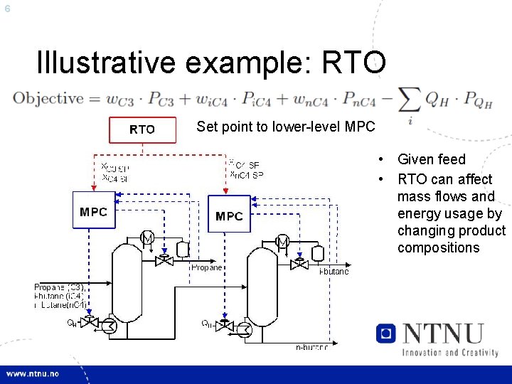
6 Illustrative example: RTO Set point to lower-level MPC • Given feed • RTO can affect mass flows and energy usage by changing product compositions

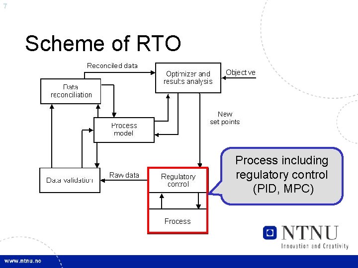
7 Scheme of RTO Process including regulatory control (PID, MPC)

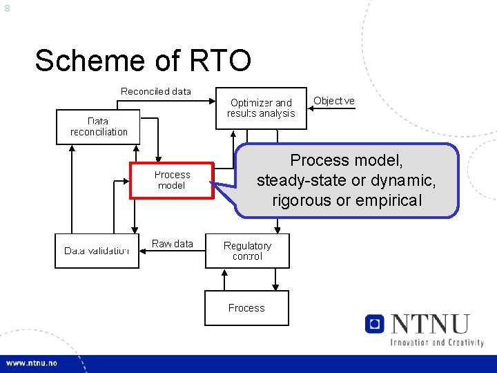
8 Scheme of RTO Process model, steady-state or dynamic, rigorous or empirical

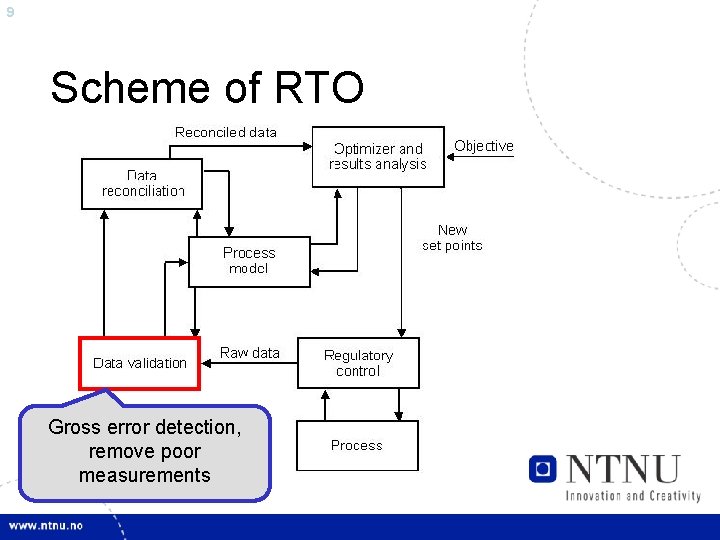
9 Scheme of RTO Gross error detection, remove poor measurements

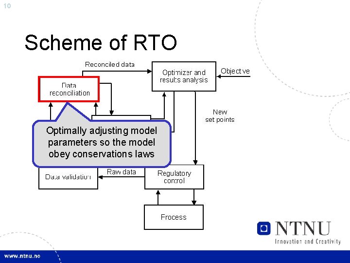
10 Scheme of RTO Optimally adjusting model parameters so the model obey conservations laws

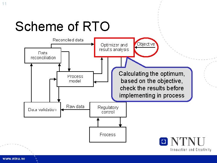
11 Scheme of RTO Calculating the optimum, based on the objective, check the results before implementing in process

12 Fundamental issue: which plants will benefit from an RTO? • Key factors: – Additional adjustable optimization variables exist (degrees of freedom) – Profit changes significantly when optimization variables are changed – Disturbances occurs frequently enough for real-time adjustment to be required – Optimality can not be achieved by constant set points (or other standard procedures) Forbes et. al. , (2006)

13 Outline • • Scope of the presentation Introduction to real-time optimization (RTO) scheme Steady-state RTO with dynamic models “Simplified RTO” Industrial case Summary

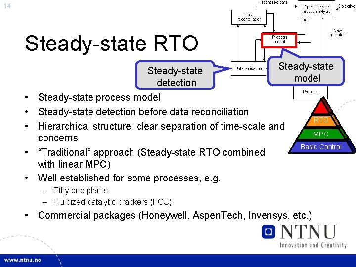
14 Steady-state RTO Steady-state detection Steady-state model • Steady-state process model • Steady-state detection before data reconciliation • Hierarchical structure: clear separation of time-scale and concerns • “Traditional” approach (Steady-state RTO combined with linear MPC) • Well established for some processes, e. g. RTO MPC Basic Control – Ethylene plants – Fluidized catalytic crackers (FCC) • Commercial packages (Honeywell, Aspen. Tech, Invensys, etc. )

15 Weaknesses with steady-state RTO • Do not handle transient plant operation – Continuous process with frequent changes in feed, product specifications, market disturbances, slow dynamics/long settling time – Continuous with frequent grade transitions – Batch processes – Cyclic operations • Force variables to fixed set points, may not utilize all degrees of freedom • A steady-state optimization layer and a control layer may lead to model inconsistency • A dynamic model can be more appropriate for the optimization task to reduce the gap between control and optimization

16 Outline • • Scope of the presentation Introduction to real-time optimization (RTO) scheme Steady-state RTO with dynamic models “Simplified RTO” Industrial case Summary

17 Optimization = “find the target” Control = “stay at the target” • Steady-state RTO: – MPC with dynamic models to control – RTO with steady-state models to optimize in separate layers • Optimization with dynamic models: – [N]MPC with dynamic models – RTO with dynamic models (D-RTO) what is the difference? • No clear separation if [N]MPC consider economy (which it often does implicitly) RTO or D-RTO or [N]MPC?

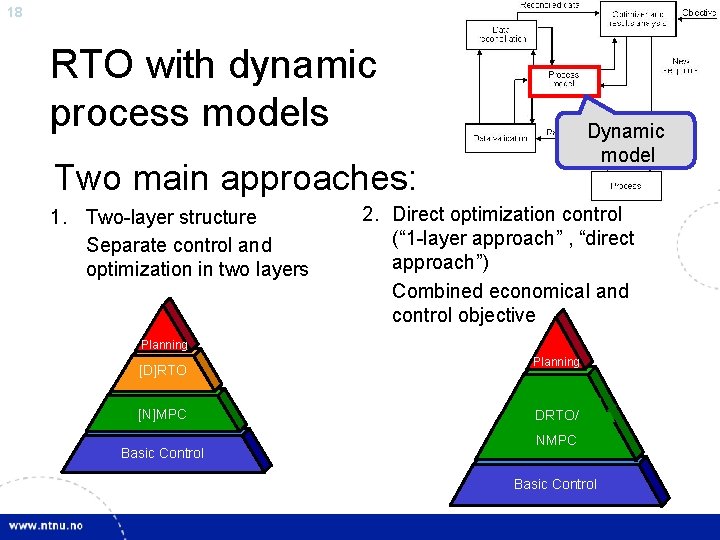
18 RTO with dynamic process models Dynamic model Two main approaches: 1. Two-layer structure Separate control and optimization in two layers 2. Direct optimization control (“ 1 -layer approach” , “direct approach”) Combined economical and control objective Planning [D]RTO [N]MPC Basic Control Planning DRTO/ NMPC Basic Control

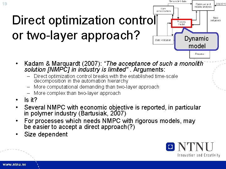
19 Direct optimization control or two-layer approach? Dynamic model • Kadam & Marquardt (2007): “The acceptance of such a monolith solution [NMPC] in industry is limited”. Arguments: – Direct optimization control breaks with the established time-scale decomposition in the automation hierarchy – More computational demanding than two-layer approach – More complex than two-layer approach • Is it? • Several NMPC with economic objective is reported, in particular in polymer industry (Bartusiak, 2007) • For processes which needs NMPC with rigorous models, may be easier to accept a direct approach(? ) • Size dependent

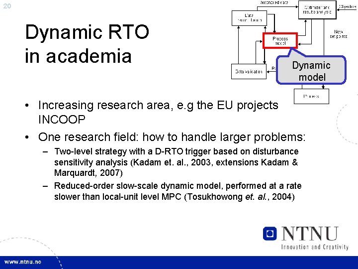
20 Dynamic RTO in academia Dynamic model • Increasing research area, e. g the EU projects INCOOP • One research field: how to handle larger problems: – Two-level strategy with a D-RTO trigger based on disturbance sensitivity analysis (Kadam et. al. , 2003, extensions Kadam & Marquardt, 2007) – Reduced-order slow-scale dynamic model, performed at a rate slower than local-unit level MPC (Tosukhowong et. al. , 2004)

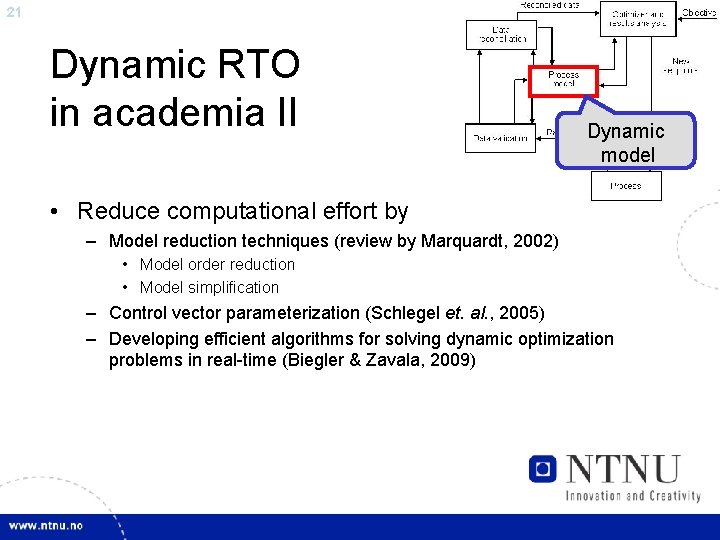
21 Dynamic RTO in academia II Dynamic model • Reduce computational effort by – Model reduction techniques (review by Marquardt, 2002) • Model order reduction • Model simplification – Control vector parameterization (Schlegel et. al. , 2005) – Developing efficient algorithms for solving dynamic optimization problems in real-time (Biegler & Zavala, 2009)

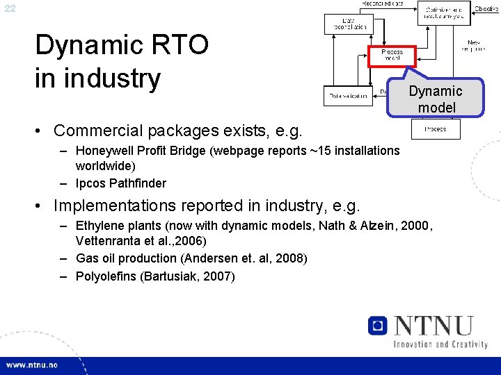
22 Dynamic RTO in industry Dynamic model • Commercial packages exists, e. g. – Honeywell Profit Bridge (webpage reports ~15 installations worldwide) – Ipcos Pathfinder • Implementations reported in industry, e. g. – Ethylene plants (now with dynamic models, Nath & Alzein, 2000, Vettenranta et al. , 2006) – Gas oil production (Andersen et. al, 2008) – Polyolefins (Bartusiak, 2007)

23 Some issues for further research • Appropriate simplification of nonlinear models • How accurate must the process model or the parameter estimates be? • Online RTO performance monitoring and diagnostics • Plantwide (dynamic) RTO – Very large scale … – or decentralized approach (with problem of sub-optimality) • Optimization algorithms – How to handle multiple minima

24 Amazing method – why is it not used everywhere? • Not available resources (people) for design, implementation and maintenance? • Not able to identify a model. . and update the model • Missing or poor measurements • Etc… • other methods possible that requires less effort?

25 Outline • • Scope of the presentation Introduction to real-time optimization (RTO) scheme Steady-state RTO with dynamic models “Simplified RTO” Industrial case Summary

26 ”Simplified RTO” • Model-free approaches like “Self-optimizing control” (Skogestad, 2000). – Find the best (=minimum loss) controlled variables to hold constant • Off-line computations • Constrained optimization realized by (linear) MPC

27 Outline • • Scope of the presentation Introduction to real-time optimization (RTO) scheme Steady-state RTO with dynamic models “Simplified RTO” Industrial case Summary

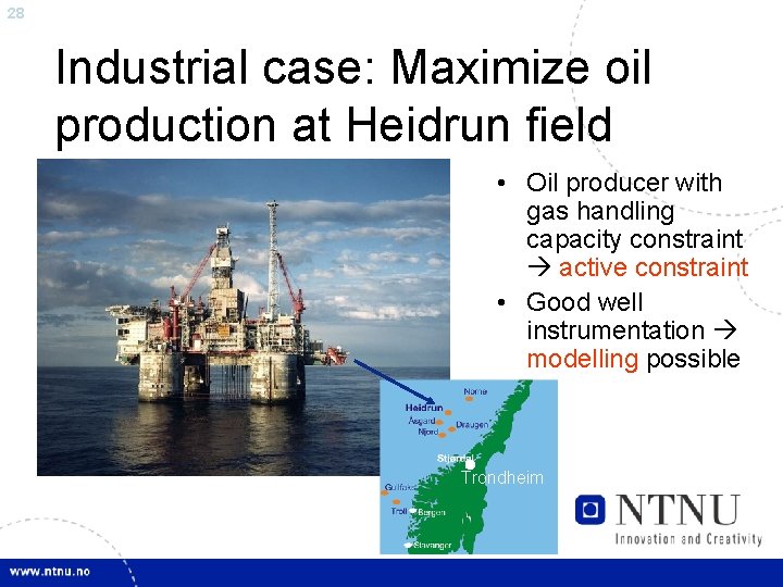
28 Industrial case: Maximize oil production at Heidrun field • Oil producer with gas handling capacity constraint active constraint • Good well instrumentation modelling possible Trondheim

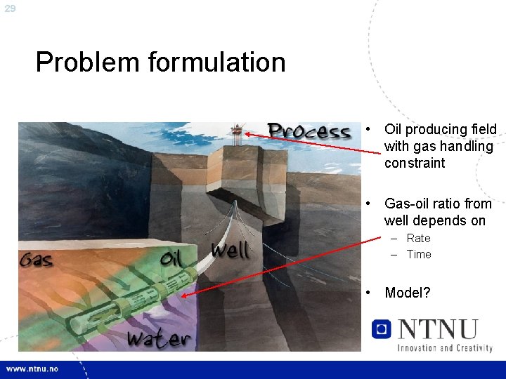
29 Problem formulation • Oil producing field with gas handling constraint • Gas-oil ratio from well depends on – Rate – Time • Model?

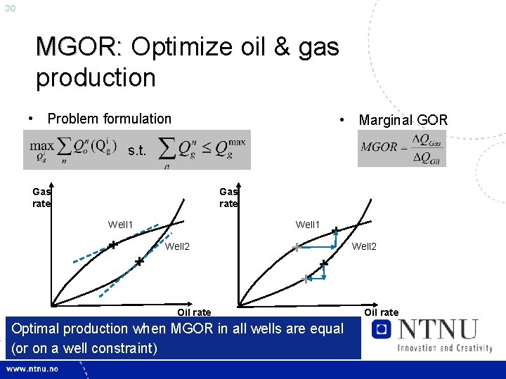
30 MGOR: Optimize oil & gas production • Problem formulation • Marginal GOR s. t. Gas rate Well 1 Well 2 Oil rate Optimal production when MGOR in all wells are equal (or on a well constraint) Well 2 Oil rate

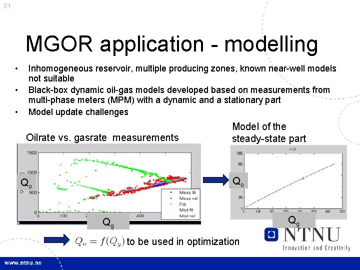
31 MGOR application - modelling • • • Inhomogeneous reservoir, multiple producing zones, known near-well models not suitable Black-box dynamic oil-gas models developed based on measurements from multi-phase meters (MPM) with a dynamic and a stationary part Model update challenges Oilrate vs. gasrate measurements Model of the steady-state part Qo Qo Qg Qg to be used in optimization

32 MGOR application • Objective: max Oil production s. t. gas constraints • Variables: gas rate allocation between wells • Maximize by setting a high, unreachable set point on oil rate with lower priority than constraints Well • Obtain “RTO” with experimental models and solved with MPC

33 Outline • • Scope of the presentation Introduction to real-time optimization (RTO) scheme Steady-state RTO with dynamic models “Simplified RTO” Industrial research case Summary

34 Summary • Two main trends: 1. RTO with dynamic models • • Extensive research Technology used in industry 2. “Simplified RTO” as a competitive approach • • Favorable if model-free approach is possible MPC with a simplified objective function

35 Acknowledgement • Bjørn Glemmestad, Borealis • Cybernetica (Tor Steinar Schei , Svein Olav Hauger, Pål Kittilsen) • Tore Lid, Statoil. Hydro • Statoil. Hydro Research Centre Trondheim & Porsgrunn (many of them) • Department of Chemical Engineering (many of them)

36 Selected references • • Andersen, T. R. , A-K. Ipsen, J. R. Kristensen, M. Fredriksen and S. Strand (2008). Controlling gas oil production and blending via MPC and dynamic RTO. In: ERTC Asset Maximisation Conference. Bartusiak, R. D. (2007). Assessment and Future Directions of Nonlinear Model Predictive Control. Chap. NLMPC: A Platform for Optimal Control of Feed- or Product-Flexible Manufacturing, pp. 367– 381. Springer Vorlag Cutler, C. R. and R. T. Perry (1983). Real time optimization with multivariable control is required to maximize profits. Comput. Chem. Eng. 7(5), 663– 667. Engell, S. (2007). Feedback control for optimal process operation. J. Proc. Control 17, 203– 219. Forbes, J. F. , T. E. Marlin and W. S. Yip (2006). Real-time optimization: Status, issues and opportunities. In: Encyclopedia of Chemical Processing (Sunggyu Lee, Ed. ). Vol. 1. pp. 2585– 2598. Taylor & Francis. Honeywell webpage: http: //hpsweb. honeywell. com/Cultures/en. US/Products/Control. Applications/Advanced. Control. Optimization/default. htm Jäschke, J. E. P. and Skogestad, S. (2009). Optimally Invariant Variable Combinations for Nonlinear Systems. To be published at ADCHEM 2009

37 Selected references II • • • Kadam, J. and W. Marquardt (2007). Integration of economical optimization and control for intentionally transient process operation. In: Assessment and Future Directions of Nonlinear Model Predictive Control (Rolf Findeisen, Frank Allgwer and Lorenz Biegler, Eds. ). pp. 419– 434. Springer Berlin / Heidelberg. Mercangöz, M. and F. J. Doyle III (2008). Real-time optimization of the pulp mill benchmark problem. Comput. Chem. Eng. 32, 789– 804. Nath, R. and Z. Alzein (2000). On-line dynamic optimization of olefins plants. Comput. Chem. Eng. 24, 533– 538. Saputelli et al. (2003), Promoting real-time optimization of hydrocarbon producing systems, Offshore Europe, Aberdeen, U. K. Skogestad, S. (2000). Plantwide control: the search for the self-optimizing control structure. J. Process Control. 10, p. 487 -507 Young, R. E. (2006). Petroleum refining process control and real-time optimization. IEEE Control Systems Magazine. 26(6), 73– 83.