1 Practicum on Solar Radio Instrumentation Tim Bastian

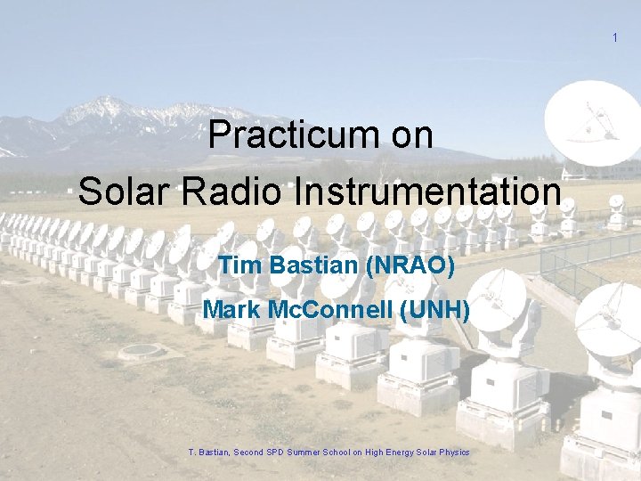
1 Practicum on Solar Radio Instrumentation Tim Bastian (NRAO) Mark Mc. Connell (UNH) T. Bastian, Second SPD Summer School on High Energy Solar Physics

Why observe the Sun at radio wavelengths? • Solar emission at radio wavelengths provides unique diagnostics for physical parameters of interest and their evolution in time and space - thermal free-free - nonthermal gyrosynchrotron - thermal gyroresonance - plasma radiation - exotica B(r), T(r, t), f(r, p, q, t) • Radio emission probes both optically thick and optically thin regimes • Radio emission probes both active and quiet phenomena • Radio emission probes all layers of the solar atmosphere from the temperature minimum to the interplanetary medium - temperature minimum to middle corona (ground) - middle corona to IPM (space) • Radio waves can be observed with high angular (arcsec), temporal (ms), and spectral resolution (k. Hz) T. Bastian, Second SPD Summer School on High Energy Solar Physics 2

Preliminaries • • • No RF lab at NRH No easy way to transport receivers and test equipment to UNH However, UNH has a Small Radio Telescope (SRT) Therefore, we’ll do things in two parts today: 1. I will present basic concepts relevant to radio instrumentation (science issues and data analysis are deferred to my other two lectures) 2. We will then use the UNH SRT remotely to observe the Sun (Mark Mc. Connell) T. Bastian, Second SPD Summer School on High Energy Solar Physics 3

Practicum on Solar Radio Instrumentation • The radio spectrum and its uses • Terminology and some important concepts • Overview of instrumentation on the ground and space - antennas and receivers - single dish observing - interferometry - Fourier synthesis imaging • Examples - radiometry and polarimetry - broadband spectroscopy - interferometry - Fourier synthesis imaging • Using the UNH SRT T. Bastian, Second SPD Summer School on High Energy Solar Physics 4

5 T. Bastian, Second SPD Summer School on High Energy Solar Physics

tbastian@nrao. edu T. Bastian, Second SPD Summer School on High Energy Solar Physics 6

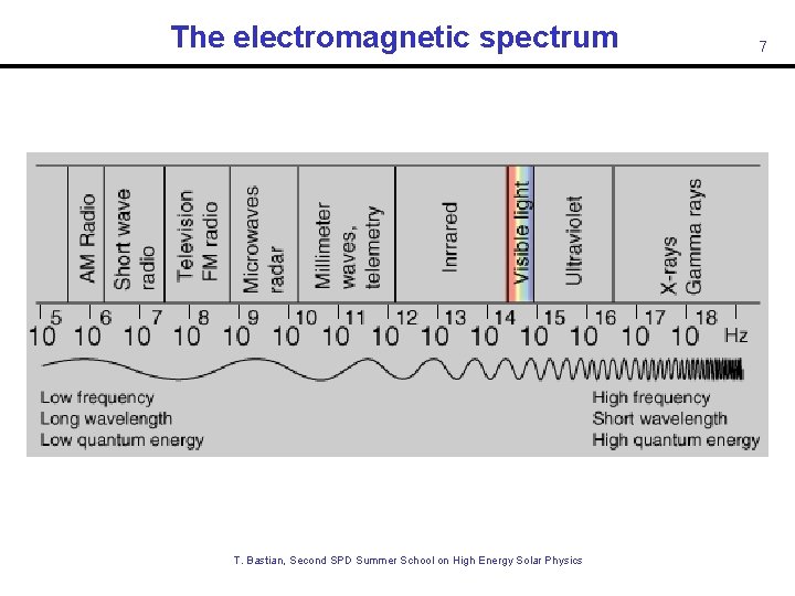
The electromagnetic spectrum T. Bastian, Second SPD Summer School on High Energy Solar Physics 7

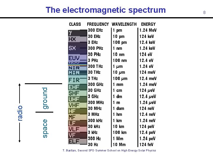
ground space radio The electromagnetic spectrum T. Bastian, Second SPD Summer School on High Energy Solar Physics 8

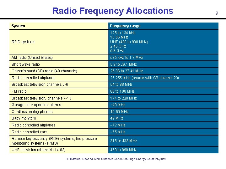
Radio Frequency Allocations System Frequency range RFID systems 125 to 134 k. Hz 13. 56 MHz UHF (400 to 930 MHz) 2. 45 GHz 5. 8 GHz AM radio (United States) 535 k. Hz to 1. 7 MHz Short wave radio 5. 9 to 26. 1 MHz Citizen's band (CB) radio (40 channels) 26. 96 to 27. 41 MHz Radio controlled airplanes 27. 255 MHz (shared with CB channel 23) Broadcast television channels 2 -6 54 to 88 MHz FM radio 88 to 108 MHz Broadcast television, channels 7 -13 174 to 220 MHz Garage door openers, alarms ~40 MHz Cordless analog phones 40 -50 MHz Baby monitors 49 MHz Radio controlled airplanes ~72 MHz Radio controlled cars ~75 MHz Remote keyless entry (RKE) systems, tire pressure monitoring systems (TPMS) 315 or 433 MHz UHF television (channels 14 -83) 470 to 890 MHz T. Bastian, Second SPD Summer School on High Energy Solar Physics 9

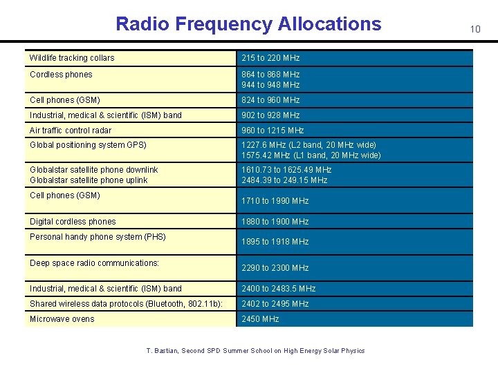
Radio Frequency Allocations Wildlife tracking collars 215 to 220 MHz Cordless phones 864 to 868 MHz 944 to 948 MHz Cell phones (GSM) 824 to 960 MHz Industrial, medical & scientific (ISM) band 902 to 928 MHz Air traffic control radar 960 to 1215 MHz Global positioning system GPS) 1227. 6 MHz (L 2 band, 20 MHz wide) 1575. 42 MHz (L 1 band, 20 MHz wide) Globalstar satellite phone downlink Globalstar satellite phone uplink 1610. 73 to 1625. 49 MHz 2484. 39 to 249. 15 MHz Cell phones (GSM) 1710 to 1990 MHz Digital cordless phones 1880 to 1900 MHz Personal handy phone system (PHS) Deep space radio communications: 1895 to 1918 MHz 2290 to 2300 MHz Industrial, medical & scientific (ISM) band 2400 to 2483. 5 MHz Shared wireless data protocols (Bluetooth, 802. 11 b): 2402 to 2495 MHz Microwave ovens 2450 MHz T. Bastian, Second SPD Summer School on High Energy Solar Physics 10

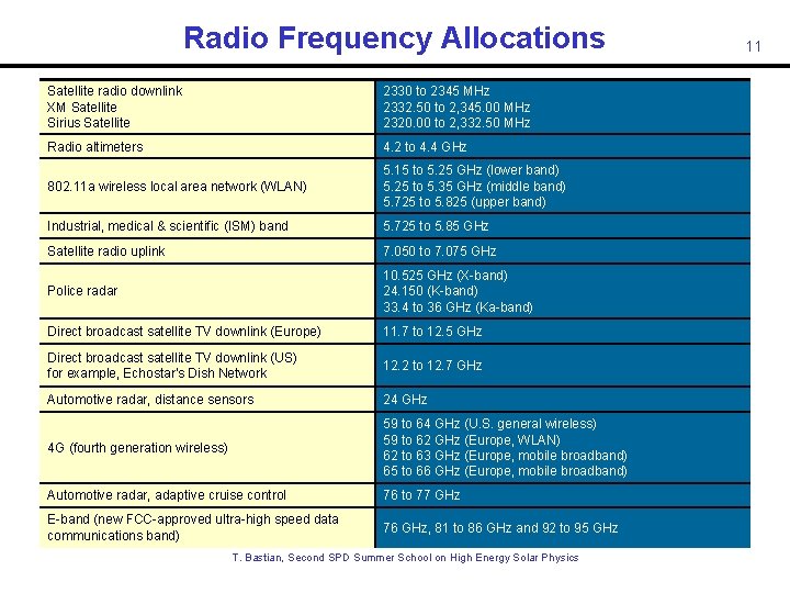
Radio Frequency Allocations Satellite radio downlink XM Satellite Sirius Satellite 2330 to 2345 MHz 2332. 50 to 2, 345. 00 MHz 2320. 00 to 2, 332. 50 MHz Radio altimeters 4. 2 to 4. 4 GHz 802. 11 a wireless local area network (WLAN) 5. 15 to 5. 25 GHz (lower band) 5. 25 to 5. 35 GHz (middle band) 5. 725 to 5. 825 (upper band) Industrial, medical & scientific (ISM) band 5. 725 to 5. 85 GHz Satellite radio uplink 7. 050 to 7. 075 GHz Police radar 10. 525 GHz (X-band) 24. 150 (K-band) 33. 4 to 36 GHz (Ka-band) Direct broadcast satellite TV downlink (Europe) 11. 7 to 12. 5 GHz Direct broadcast satellite TV downlink (US) for example, Echostar's Dish Network 12. 2 to 12. 7 GHz Automotive radar, distance sensors 24 GHz 4 G (fourth generation wireless) 59 to 64 GHz (U. S. general wireless) 59 to 62 GHz (Europe, WLAN) 62 to 63 GHz (Europe, mobile broadband) 65 to 66 GHz (Europe, mobile broadband) Automotive radar, adaptive cruise control 76 to 77 GHz E-band (new FCC-approved ultra-high speed data communications band) 76 GHz, 81 to 86 GHz and 92 to 95 GHz T. Bastian, Second SPD Summer School on High Energy Solar Physics 11

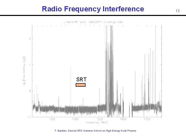
Radio Frequency Interference SRT T. Bastian, Second SPD Summer School on High Energy Solar Physics 12

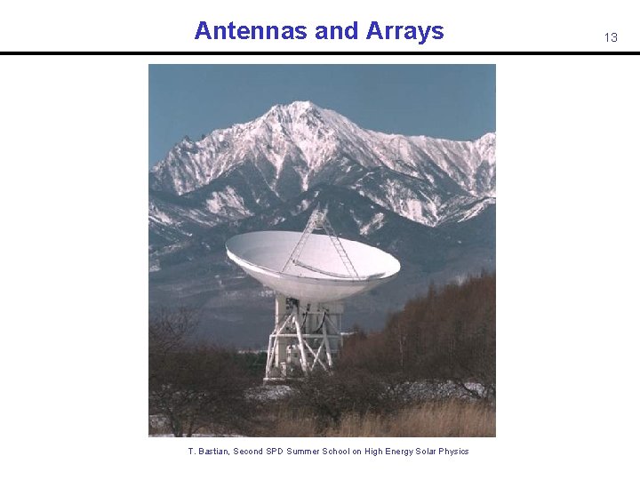
Antennas and Arrays T. Bastian, Second SPD Summer School on High Energy Solar Physics 13

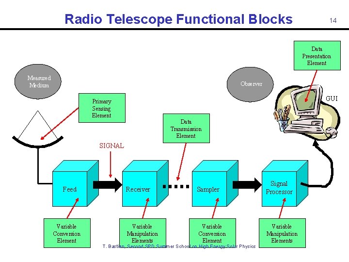
Radio Telescope Functional Blocks 14 Data Presentation Element Measured Medium Observer GUI Primary Sensing Element Data Transmission Element SIGNAL Feed Variable Conversion Element Receiver Variable Manipulation Elements Sampler Variable Conversion Element T. Bastian, Second SPD Summer School on High Energy Solar Physics Signal Processor Variable Manipulation Elements

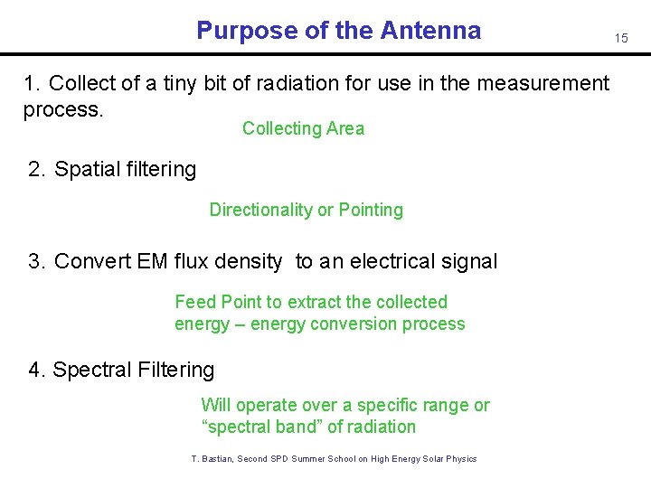
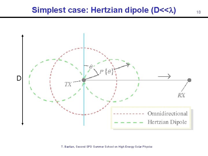
Purpose of the Antenna 1. Collect of a tiny bit of radiation for use in the measurement process. Collecting Area 2. Spatial filtering Directionality or Pointing 3. Convert EM flux density to an electrical signal Feed Point to extract the collected energy – energy conversion process 4. Spectral Filtering Will operate over a specific range or “spectral band” of radiation T. Bastian, Second SPD Summer School on High Energy Solar Physics 15

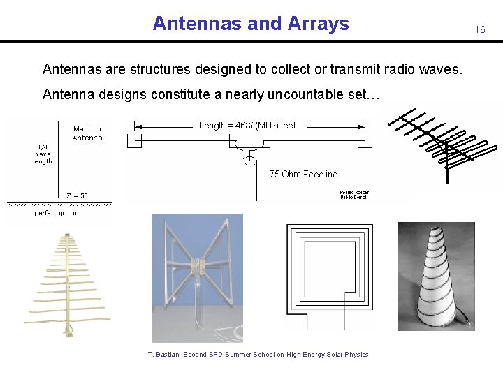
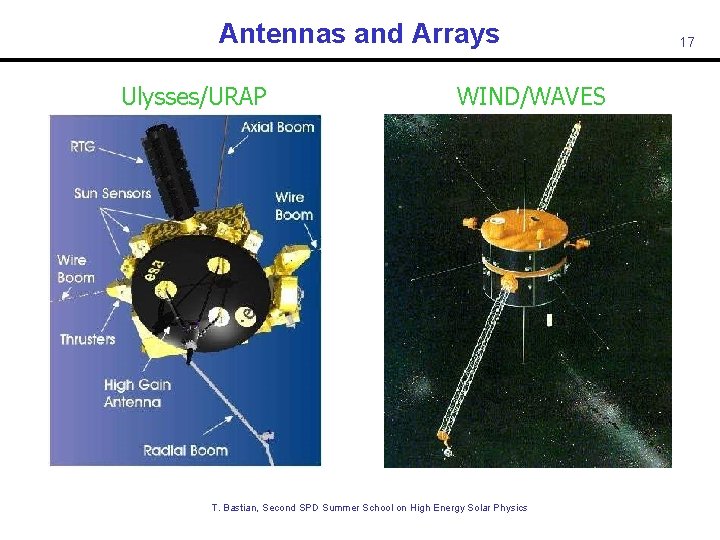
Antennas and Arrays Antennas are structures designed to collect or transmit radio waves. Antenna designs constitute a nearly uncountable set… T. Bastian, Second SPD Summer School on High Energy Solar Physics 16

Antennas and Arrays Ulysses/URAP WIND/WAVES T. Bastian, Second SPD Summer School on High Energy Solar Physics 17

Simplest case: Hertzian dipole (D<<l) D T. Bastian, Second SPD Summer School on High Energy Solar Physics 18

Antennas and Arrays The design of a particular antenna must be matched to the problem at hand. Low frequency antennas ( < few x 100 MHz) may employ some variant of a dipole or phased dipole array since their effective area is proportional to l 2. At higher frequencies, signal is collected with a mirror that most often takes the form of a parabolic reflector of diameter D >> l. This focuses radiation on a feed that couples the radiation to electronics that amplify the signal. For our purposes, we will consider a conventional parabolic antenna in order to illustrate some basic concepts before discussing interferometry and Fourier synthesis imaging (which is basically what RHESSI does). T. Bastian, Second SPD Summer School on High Energy Solar Physics 19

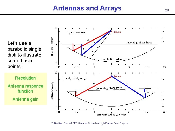
Antennas and Arrays Let’s use a parabolic single dish to illustrate some basic points. Resolution Antenna response function Antenna gain T. Bastian, Second SPD Summer School on High Energy Solar Physics 20

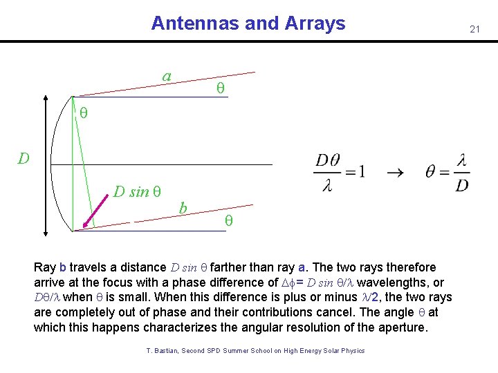
Antennas and Arrays a q q D D sin q b q Ray b travels a distance D sin q farther than ray a. The two rays therefore arrive at the focus with a phase difference of Df= D sin q/l wavelengths, or Dq/l when q is small. When this difference is plus or minus l/2, the two rays are completely out of phase and their contributions cancel. The angle q at which this happens characterizes the angular resolution of the aperture. T. Bastian, Second SPD Summer School on High Energy Solar Physics 21

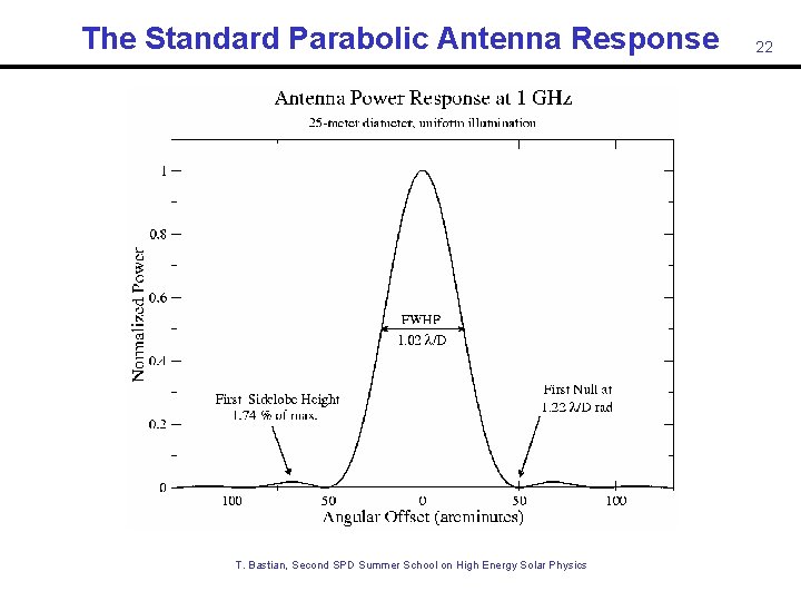
The Standard Parabolic Antenna Response T. Bastian, Second SPD Summer School on High Energy Solar Physics 22

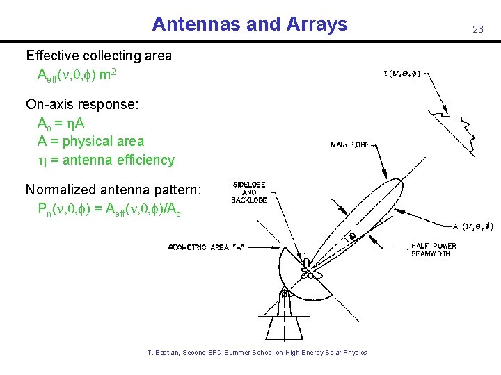
Antennas and Arrays Effective collecting area Aeff( , q, f) m 2 On-axis response: Ao = A A = physical area = antenna efficiency Normalized antenna pattern: Pn( , q, f) = Aeff( , q, f)/Ao T. Bastian, Second SPD Summer School on High Energy Solar Physics 23

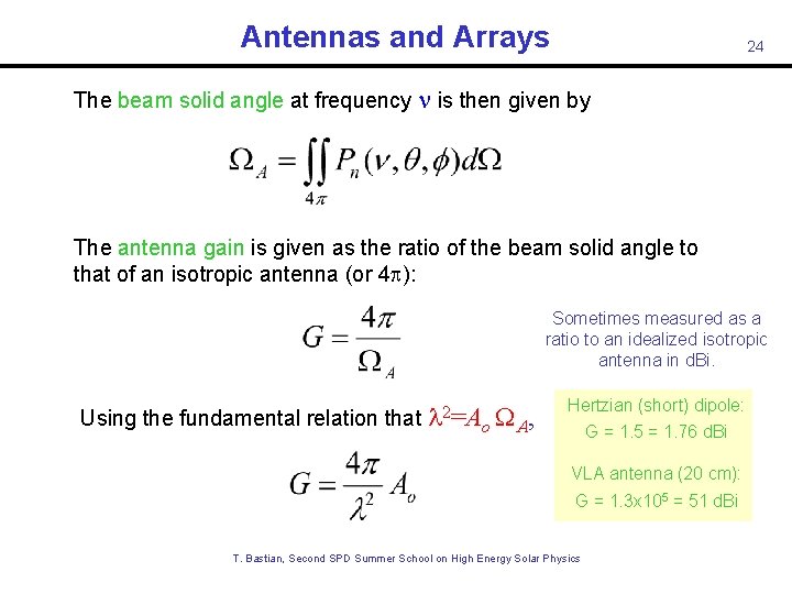
Antennas and Arrays 24 The beam solid angle at frequency is then given by The antenna gain is given as the ratio of the beam solid angle to that of an isotropic antenna (or 4 p): Sometimes measured as a ratio to an idealized isotropic antenna in d. Bi. Using the fundamental relation that l 2=Ao WA, Hertzian (short) dipole: G = 1. 5 = 1. 76 d. Bi VLA antenna (20 cm): G = 1. 3 x 105 = 51 d. Bi T. Bastian, Second SPD Summer School on High Energy Solar Physics

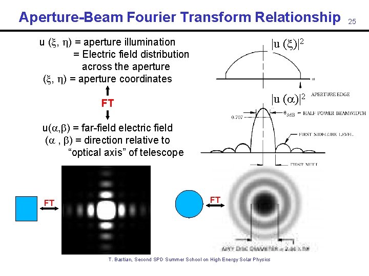
Aperture-Beam Fourier Transform Relationship u ( , ) = aperture illumination = Electric field distribution across the aperture ( , ) = aperture coordinates |u ( )|2 FT u( , ) = far-field electric field ( , ) = direction relative to “optical axis” of telescope FT FT T. Bastian, Second SPD Summer School on High Energy Solar Physics 25

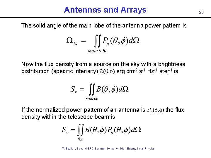
Antennas and Arrays The solid angle of the main lobe of the antenna power pattern is Now the flux density from a source on the sky with a brightness distribution (specific intensity) B(q, f) erg cm-2 s-1 Hz-1 ster-1 is If the normalized power pattern of an antenna is Pn(q, f) the flux density within the telescope beam is T. Bastian, Second SPD Summer School on High Energy Solar Physics 26

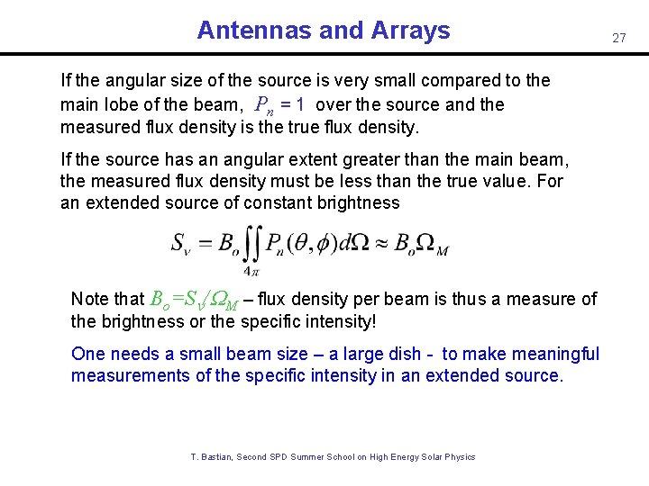
Antennas and Arrays If the angular size of the source is very small compared to the main lobe of the beam, Pn = 1 over the source and the measured flux density is the true flux density. If the source has an angular extent greater than the main beam, the measured flux density must be less than the true value. For an extended source of constant brightness Note that Bo=S /WM – flux density per beam is thus a measure of the brightness or the specific intensity! One needs a small beam size – a large dish - to make meaningful measurements of the specific intensity in an extended source. T. Bastian, Second SPD Summer School on High Energy Solar Physics 27

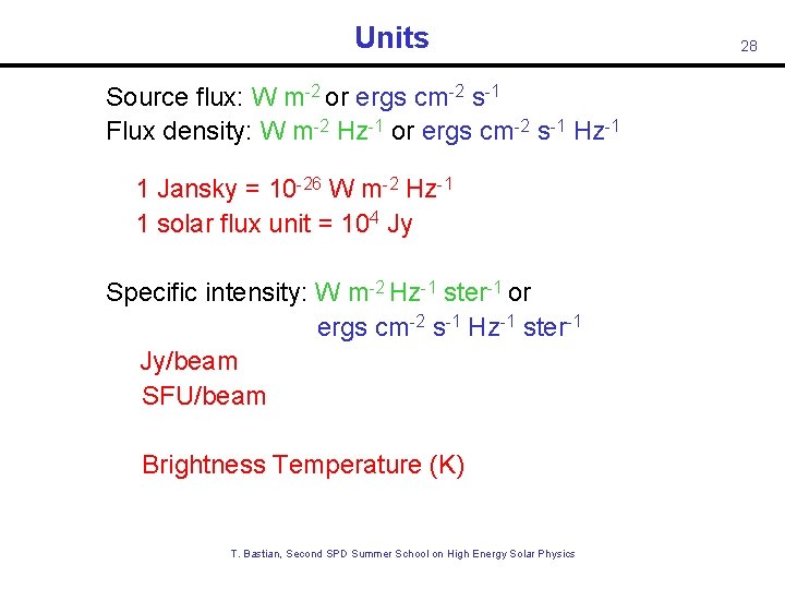
Units Source flux: W m-2 or ergs cm-2 s-1 Flux density: W m-2 Hz-1 or ergs cm-2 s-1 Hz-1 1 Jansky = 10 -26 W m-2 Hz-1 1 solar flux unit = 104 Jy Specific intensity: W m-2 Hz-1 ster-1 or ergs cm-2 s-1 Hz-1 ster-1 Jy/beam SFU/beam Brightness Temperature (K) T. Bastian, Second SPD Summer School on High Energy Solar Physics 28

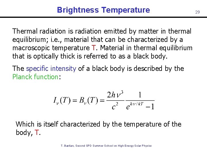
Brightness Temperature Thermal radiation is radiation emitted by matter in thermal equilibrium; i. e. , material that can be characterized by a macroscopic temperature T. Material in thermal equilibrium that is optically thick is referred to as a black body. The specific intensity of a black body is described by the Planck function: Which is itself characterized by the temperature of the body, T. T. Bastian, Second SPD Summer School on High Energy Solar Physics 29

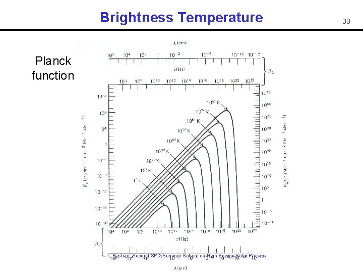
Brightness Temperature Planck function T. Bastian, Second SPD Summer School on High Energy Solar Physics 30

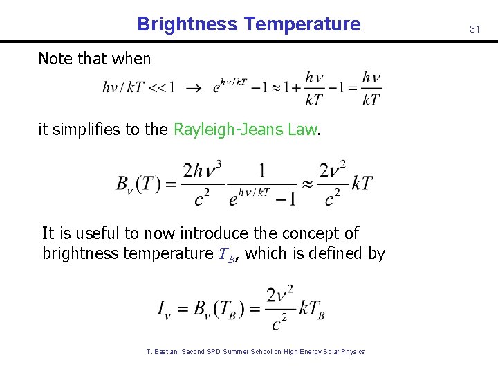
Brightness Temperature Note that when it simplifies to the Rayleigh-Jeans Law. It is useful to now introduce the concept of brightness temperature TB, which is defined by T. Bastian, Second SPD Summer School on High Energy Solar Physics 31

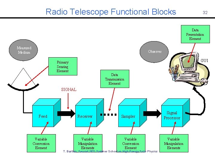
Radio Telescope Functional Blocks 32 Data Presentation Element Measured Medium Observer GUI Primary Sensing Element Data Transmission Element SIGNAL Feed Variable Conversion Element Receiver Variable Manipulation Elements Sampler Variable Conversion Element T. Bastian, Second SPD Summer School on High Energy Solar Physics Signal Processor Variable Manipulation Elements

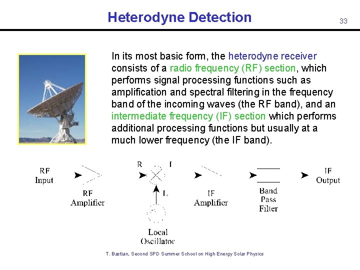
Heterodyne Detection In its most basic form, the heterodyne receiver consists of a radio frequency (RF) section, which performs signal processing functions such as amplification and spectral filtering in the frequency band of the incoming waves (the RF band), and an intermediate frequency (IF) section which performs additional processing functions but usually at a much lower frequency (the IF band). T. Bastian, Second SPD Summer School on High Energy Solar Physics 33

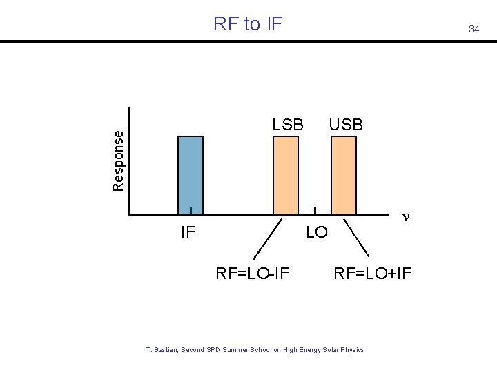
RF to IF 34 Response LSB IF USB LO RF=LO-IF RF=LO+IF T. Bastian, Second SPD Summer School on High Energy Solar Physics

A Few Performance Parameters Noise – the uncertainty in the output signal. Ideally, this noise consists of only statistical fluctuations. Linearity – the degree of which the output signal is proportional to the input photons that are collected. Dynamic range – the maximum variation in the radiation power over which the detector output represents the photon flux. Number and size of pixels – the number of picture elements that the detector can record simultaneously and the physical size of each element in the detector. Time response – the minimum interval of time over which the detector can distinguish changes in the photon arrival rate. Spectral response – the total wavelength or frequency range over which the photons can be detected with reasonable efficiency. T. Bastian, Second SPD Summer School on High Energy Solar Physics 35

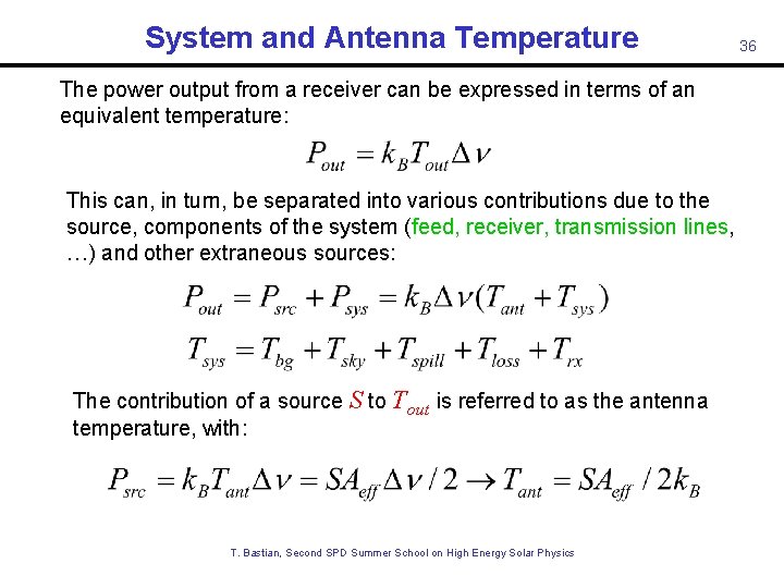
System and Antenna Temperature The power output from a receiver can be expressed in terms of an equivalent temperature: This can, in turn, be separated into various contributions due to the source, components of the system (feed, receiver, transmission lines, …) and other extraneous sources: The contribution of a source S to Tout is referred to as the antenna temperature, with: T. Bastian, Second SPD Summer School on High Energy Solar Physics 36

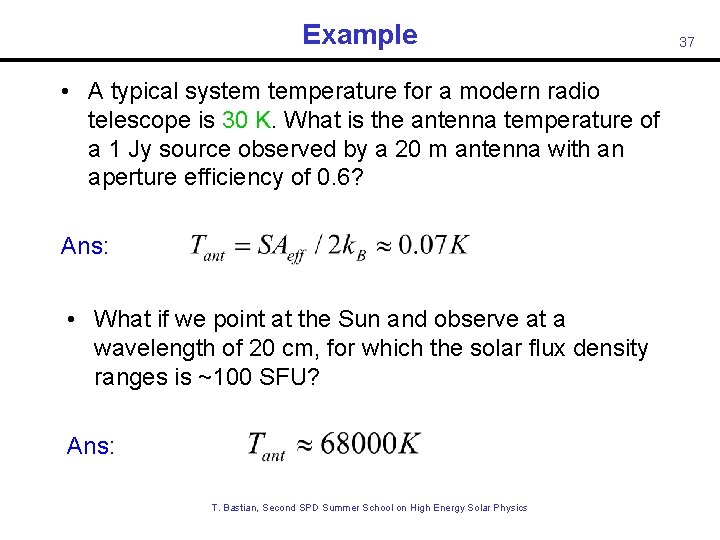
Example • A typical system temperature for a modern radio telescope is 30 K. What is the antenna temperature of a 1 Jy source observed by a 20 m antenna with an aperture efficiency of 0. 6? Ans: • What if we point at the Sun and observe at a wavelength of 20 cm, for which the solar flux density ranges is ~100 SFU? Ans: T. Bastian, Second SPD Summer School on High Energy Solar Physics 37

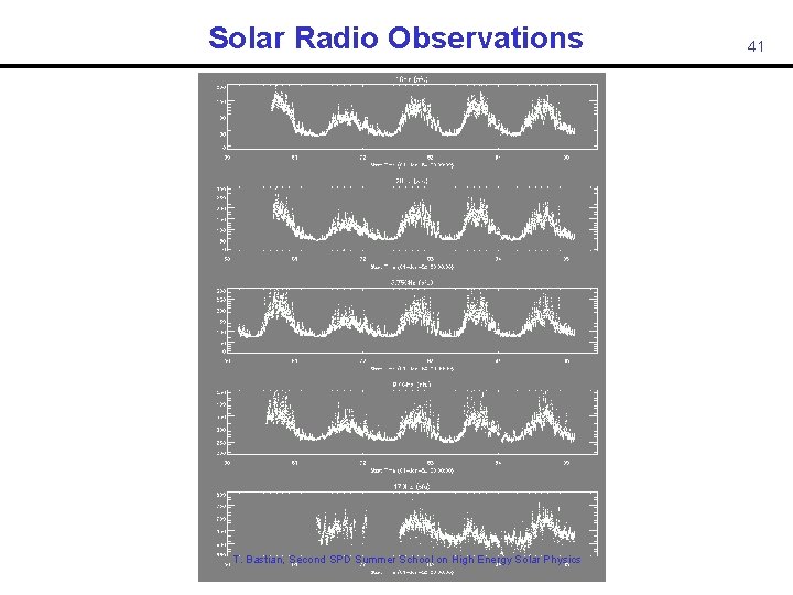
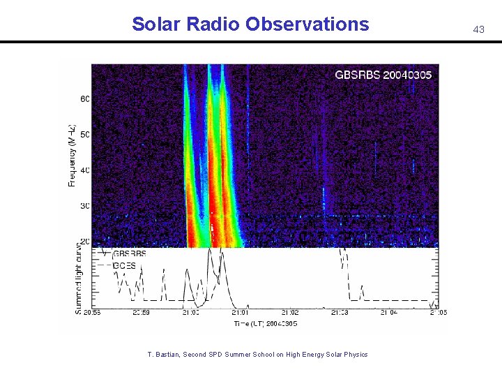
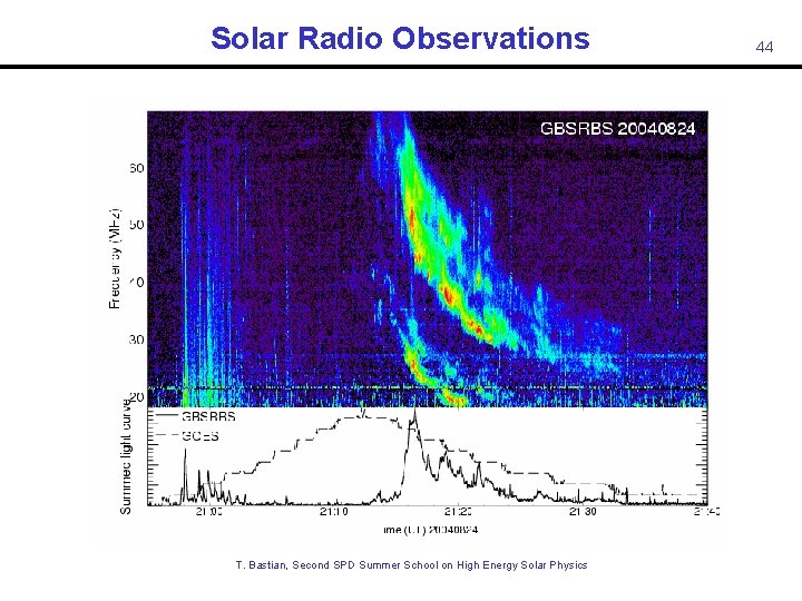
Solar Radio Observations Some Examples • Total flux monitoring • Dynamic Spectroscopy T. Bastian, Second SPD Summer School on High Energy Solar Physics 38

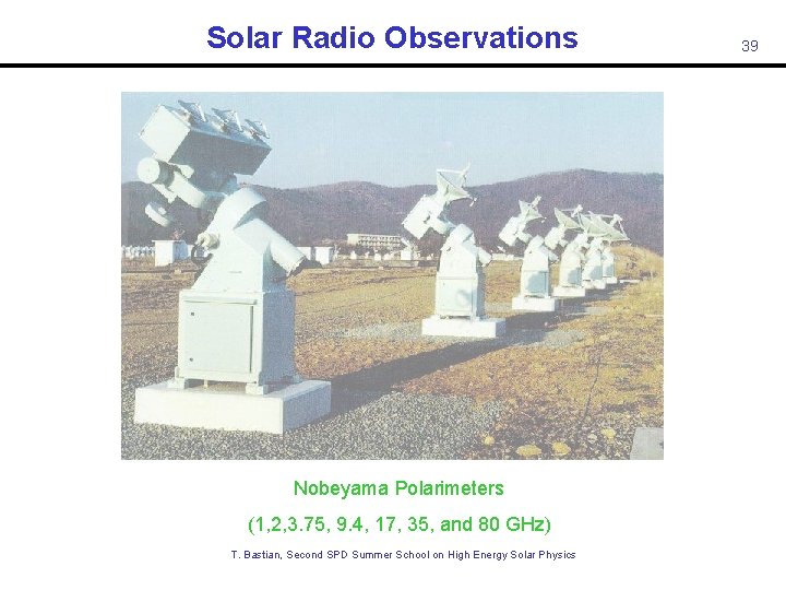
Solar Radio Observations Nobeyama Polarimeters (1, 2, 3. 75, 9. 4, 17, 35, and 80 GHz) T. Bastian, Second SPD Summer School on High Energy Solar Physics 39

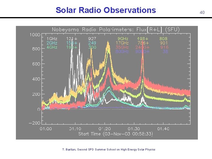
Solar Radio Observations T. Bastian, Second SPD Summer School on High Energy Solar Physics 40

Solar Radio Observations T. Bastian, Second SPD Summer School on High Energy Solar Physics 41

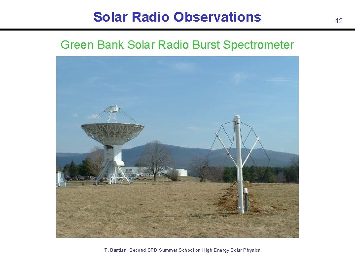
Solar Radio Observations Green Bank Solar Radio Burst Spectrometer T. Bastian, Second SPD Summer School on High Energy Solar Physics 42

Solar Radio Observations T. Bastian, Second SPD Summer School on High Energy Solar Physics 43

Solar Radio Observations T. Bastian, Second SPD Summer School on High Energy Solar Physics 44

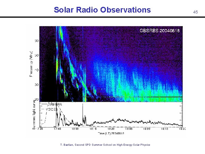
Solar Radio Observations T. Bastian, Second SPD Summer School on High Energy Solar Physics 45

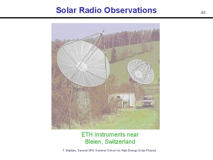
Solar Radio Observations ETH instruments near Bleien, Switzerland T. Bastian, Second SPD Summer School on High Energy Solar Physics 46

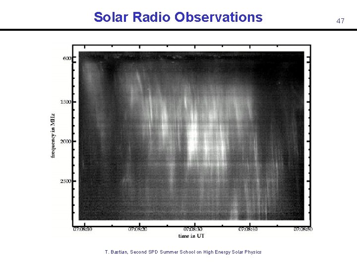
Solar Radio Observations 47 T. Bastian, Second SPD Summer School on High Energy Solar Physics Isliker & Benz 1994

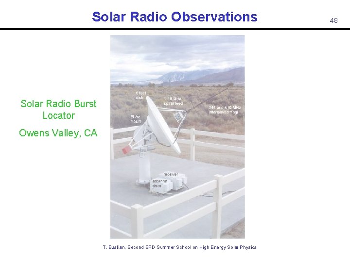
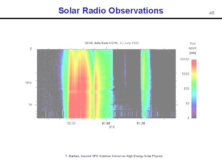
Solar Radio Observations Solar Radio Burst Locator Owens Valley, CA T. Bastian, Second SPD Summer School on High Energy Solar Physics 48

Solar Radio Observations T. Bastian, Second SPD Summer School on High Energy Solar Physics 49

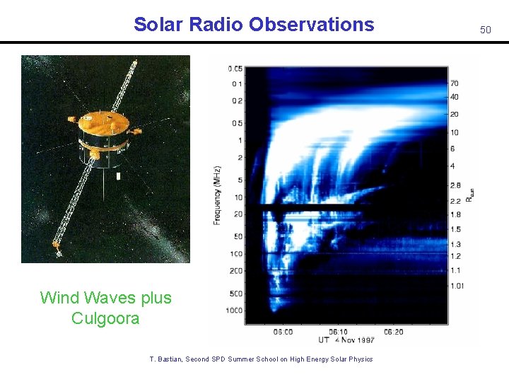
Solar Radio Observations 50 Wind Waves plus Culgoora T. Bastian, Second SPD Summer School on High Energy Solar Physics Dulk et al. 2001

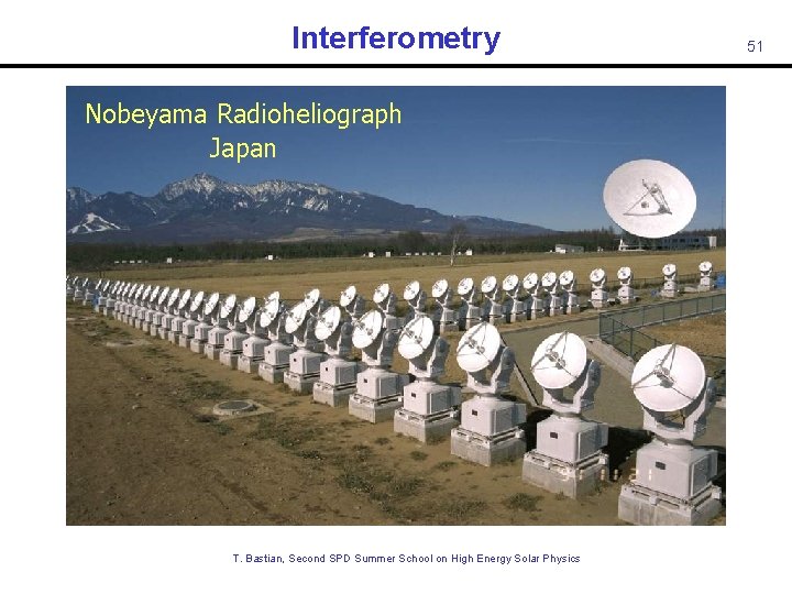
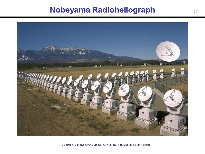
Interferometry Nobeyama Radioheliograph Japan T. Bastian, Second SPD Summer School on High Energy Solar Physics 51

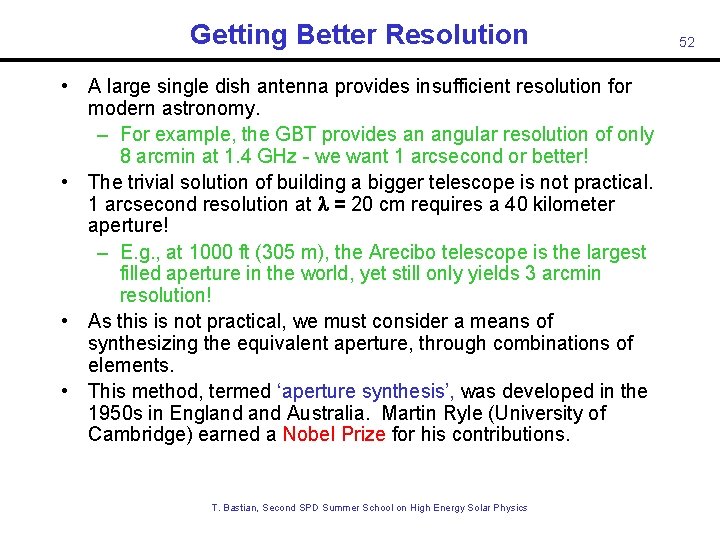
Getting Better Resolution • A large single dish antenna provides insufficient resolution for modern astronomy. – For example, the GBT provides an angular resolution of only 8 arcmin at 1. 4 GHz - we want 1 arcsecond or better! • The trivial solution of building a bigger telescope is not practical. 1 arcsecond resolution at l = 20 cm requires a 40 kilometer aperture! – E. g. , at 1000 ft (305 m), the Arecibo telescope is the largest filled aperture in the world, yet still only yields 3 arcmin resolution! • As this is not practical, we must consider a means of synthesizing the equivalent aperture, through combinations of elements. • This method, termed ‘aperture synthesis’, was developed in the 1950 s in England Australia. Martin Ryle (University of Cambridge) earned a Nobel Prize for his contributions. T. Bastian, Second SPD Summer School on High Energy Solar Physics 52

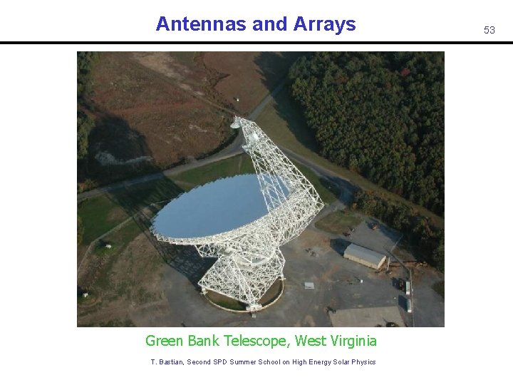
Antennas and Arrays Green Bank Telescope, West Virginia T. Bastian, Second SPD Summer School on High Energy Solar Physics 53

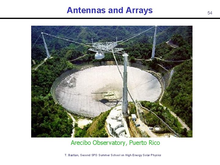
Antennas and Arrays Arecibo Observatory, Puerto Rico T. Bastian, Second SPD Summer School on High Energy Solar Physics 54

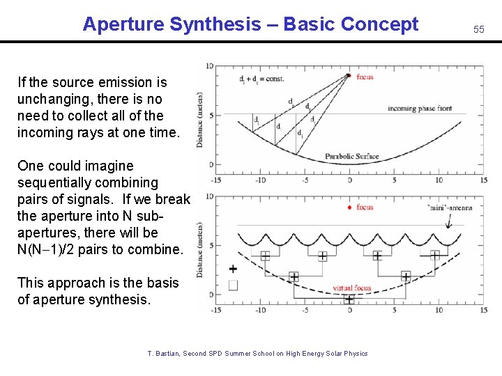
Aperture Synthesis – Basic Concept If the source emission is unchanging, there is no need to collect all of the incoming rays at one time. One could imagine sequentially combining pairs of signals. If we break the aperture into N subapertures, there will be N(N-1)/2 pairs to combine. This approach is the basis of aperture synthesis. T. Bastian, Second SPD Summer School on High Energy Solar Physics 55

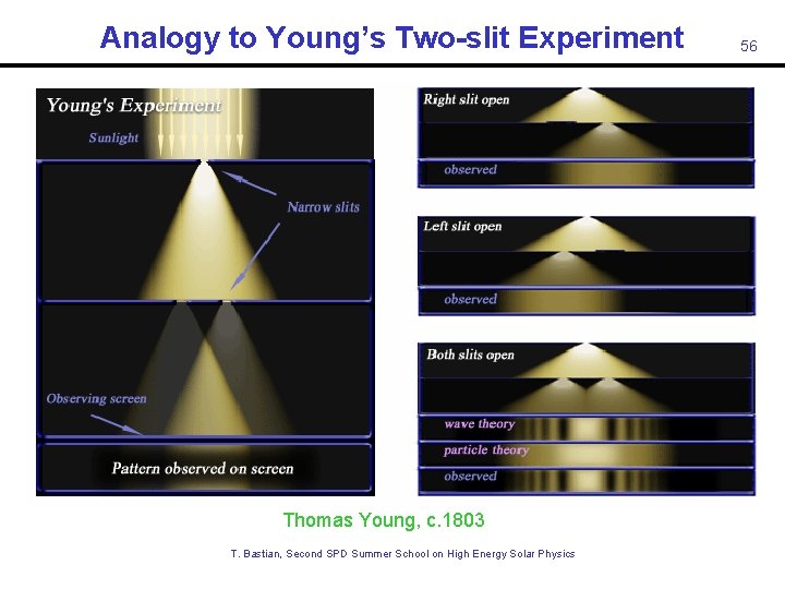
Analogy to Young’s Two-slit Experiment Thomas Young, c. 1803 T. Bastian, Second SPD Summer School on High Energy Solar Physics 56

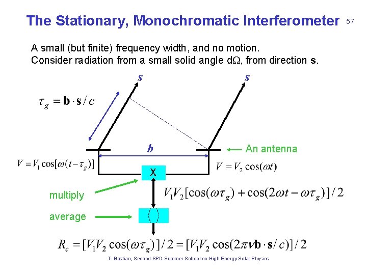
The Stationary, Monochromatic Interferometer A small (but finite) frequency width, and no motion. Consider radiation from a small solid angle d. W, from direction s. s s b An antenna X multiply average T. Bastian, Second SPD Summer School on High Energy Solar Physics 57

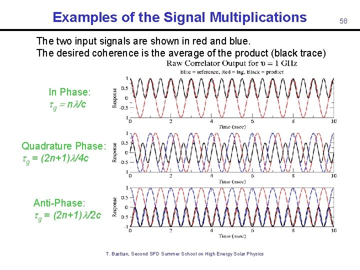
Examples of the Signal Multiplications The two input signals are shown in red and blue. The desired coherence is the average of the product (black trace) In Phase: tg = nl/c Quadrature Phase: tg = (2 n+1)l/4 c Anti-Phase: tg = (2 n+1)l/2 c T. Bastian, Second SPD Summer School on High Energy Solar Physics 58

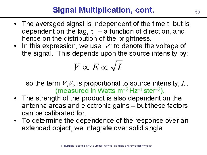
Signal Multiplication, cont. • The averaged signal is independent of the time t, but is dependent on the lag, g – a function of direction, and hence on the distribution of the brightness. • In this expression, we use ‘V’ to denote the voltage of the signal. This depends upon the source intensity by: so the term V 1 V 2 is proportional to source intensity, I. (measured in Watts m-2 Hz-1 ster-2). • The strength of the product is also dependent on the antenna areas and electronic gains – but these factors can be calibrated for. • To determine the dependence of the response over an extended object, we integrate over solid angle. T. Bastian, Second SPD Summer School on High Energy Solar Physics 59

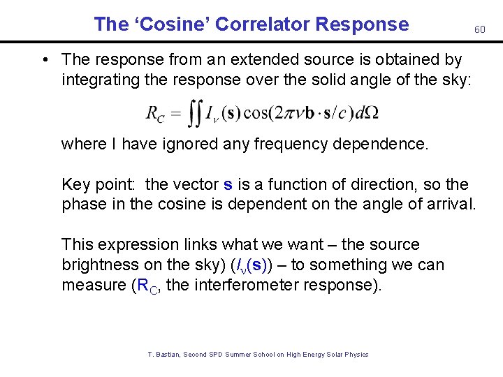
The ‘Cosine’ Correlator Response 60 • The response from an extended source is obtained by integrating the response over the solid angle of the sky: where I have ignored any frequency dependence. Key point: the vector s is a function of direction, so the phase in the cosine is dependent on the angle of arrival. This expression links what we want – the source brightness on the sky) (I (s)) – to something we can measure (RC, the interferometer response). T. Bastian, Second SPD Summer School on High Energy Solar Physics

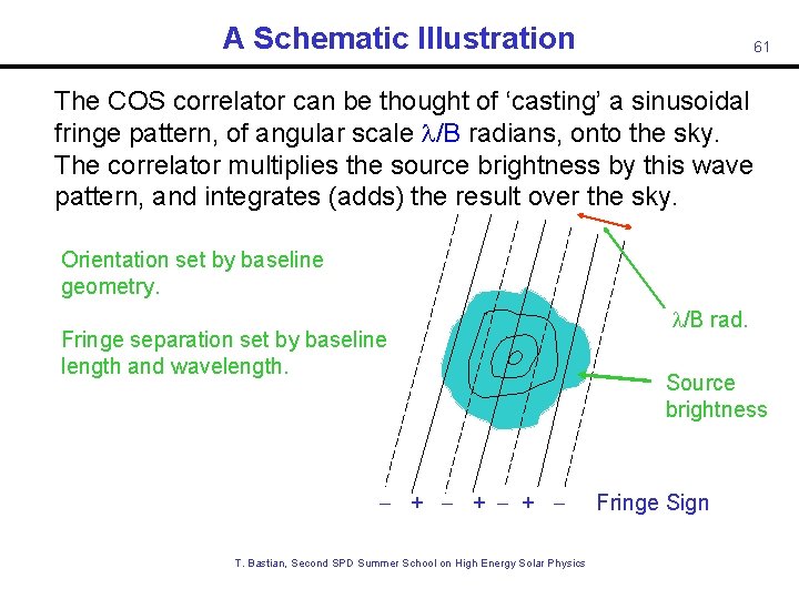
A Schematic Illustration 61 The COS correlator can be thought of ‘casting’ a sinusoidal fringe pattern, of angular scale l/B radians, onto the sky. The correlator multiplies the source brightness by this wave pattern, and integrates (adds) the result over the sky. Orientation set by baseline geometry. Fringe separation set by baseline length and wavelength. - + - + T. Bastian, Second SPD Summer School on High Energy Solar Physics l/B rad. Source brightness Fringe Sign

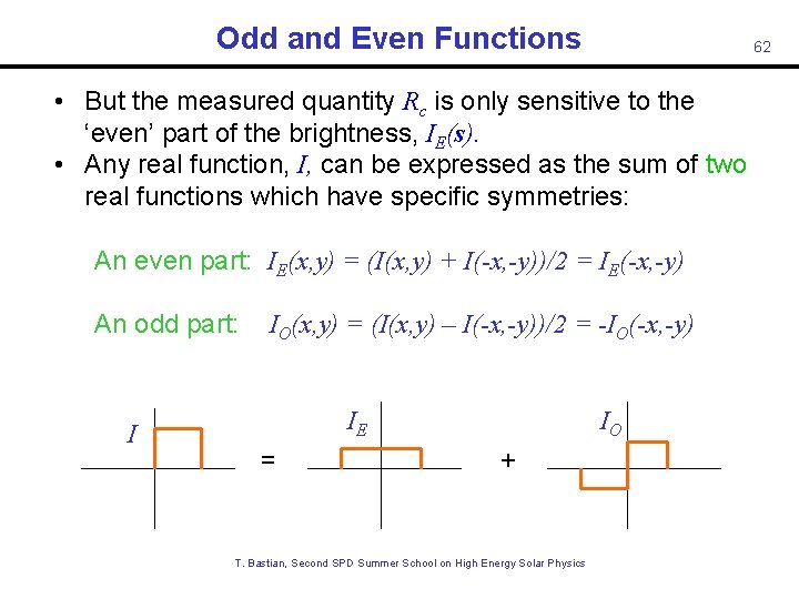
Odd and Even Functions 62 • But the measured quantity Rc is only sensitive to the ‘even’ part of the brightness, IE(s). • Any real function, I, can be expressed as the sum of two real functions which have specific symmetries: An even part: IE(x, y) = (I(x, y) + I(-x, -y))/2 = IE(-x, -y) An odd part: I IO(x, y) = (I(x, y) – I(-x, -y))/2 = -IO(-x, -y) IE = IO + T. Bastian, Second SPD Summer School on High Energy Solar Physics

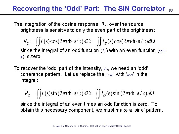
Recovering the ‘Odd’ Part: The SIN Correlator The integration of the cosine response, Rc, over the source brightness is sensitive to only the even part of the brightness: since the integral of an odd function (IO) with an even function (cos x) is zero. To recover the ‘odd’ part of the intensity, IO, we need an ‘odd’ coherence pattern. Let us replace the ‘cos’ with ‘sin’ in the integral: since the integral of an even times an odd function is zero. To obtain this necessary component, we must make a ‘sine’ pattern. T. Bastian, Second SPD Summer School on High Energy Solar Physics 63

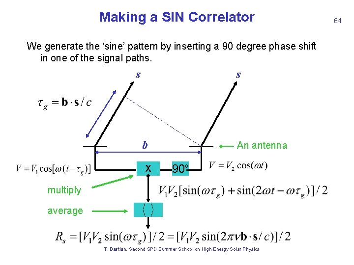
Making a SIN Correlator We generate the ‘sine’ pattern by inserting a 90 degree phase shift in one of the signal paths. s s b X An antenna 90 o multiply average T. Bastian, Second SPD Summer School on High Energy Solar Physics 64

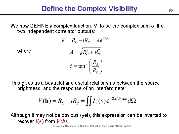
Define the Complex Visibility We now DEFINE a complex function, V, to be the complex sum of the two independent correlator outputs: where This gives us a beautiful and useful relationship between the source brightness, and the response of an interferometer: Although it may not be obvious (yet), this expression can be inverted to recover I(s) from V(b). T. Bastian, Second SPD Summer School on High Energy Solar Physics 65

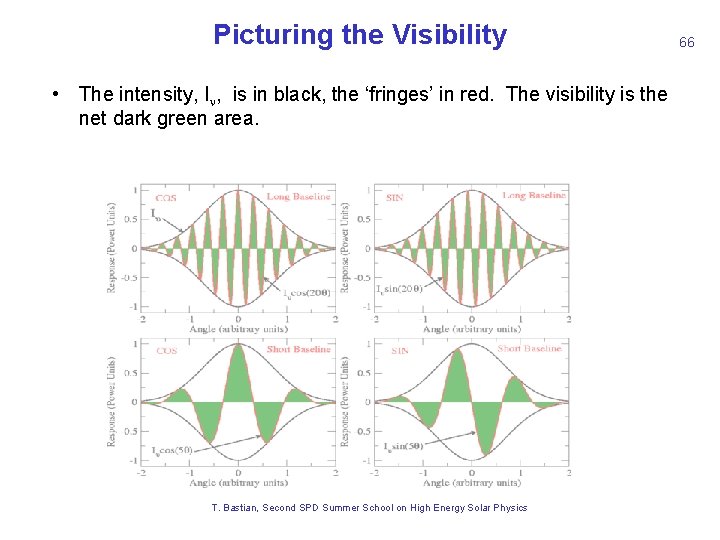
Picturing the Visibility 66 • The intensity, I , is in black, the ‘fringes’ in red. The visibility is the net dark green area. RC RS Long Baseline Short Baseline T. Bastian, Second SPD Summer School on High Energy Solar Physics

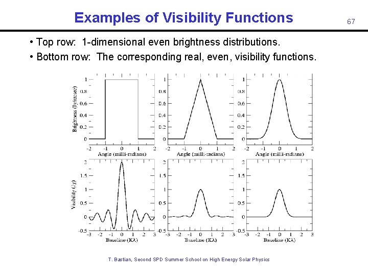
Examples of Visibility Functions • Top row: 1 -dimensional even brightness distributions. • Bottom row: The corresponding real, even, visibility functions. T. Bastian, Second SPD Summer School on High Energy Solar Physics 67

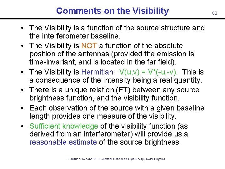
Comments on the Visibility • The Visibility is a function of the source structure and the interferometer baseline. • The Visibility is NOT a function of the absolute position of the antennas (provided the emission is time-invariant, and is located in the far field). • The Visibility is Hermitian: V(u, v) = V*(-u, -v). This is a consequence of the intensity being a real quantity. • There is a unique relation (FT) between any source brightness function, and the visibility function. • Each observation of the source with a given baseline length provides one measure of the visibility. • Sufficient knowledge of the visibility function (as derived from an interferometer) will provide us a reasonable estimate of the source brightness. T. Bastian, Second SPD Summer School on High Energy Solar Physics 68

Solar Radio Observations Some Examples • Cliff interferometer • Synthesis images • Snapshot imaging T. Bastian, Second SPD Summer School on High Energy Solar Physics 69

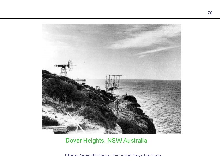
70 Dover Heights, NSW Australia T. Bastian, Second SPD Summer School on High Energy Solar Physics

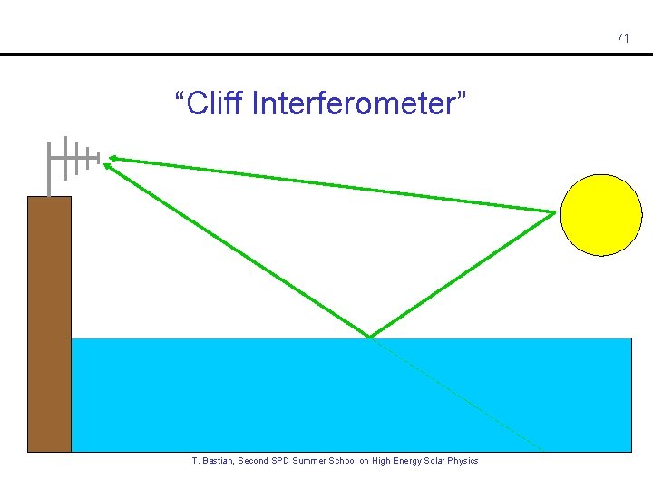
71 “Cliff Interferometer” T. Bastian, Second SPD Summer School on High Energy Solar Physics

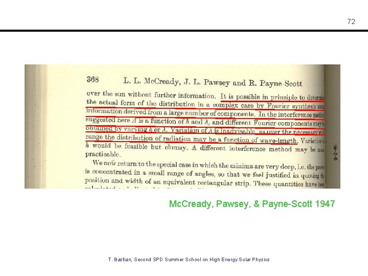
72 Mc. Cready, Pawsey, & Payne-Scott 1947 T. Bastian, Second SPD Summer School on High Energy Solar Physics

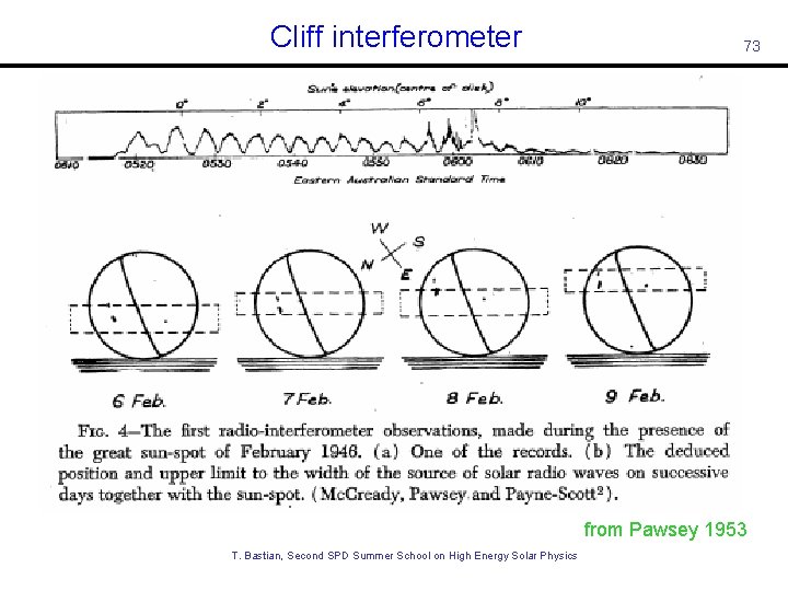
Cliff interferometer 73 from Pawsey 1953 T. Bastian, Second SPD Summer School on High Energy Solar Physics

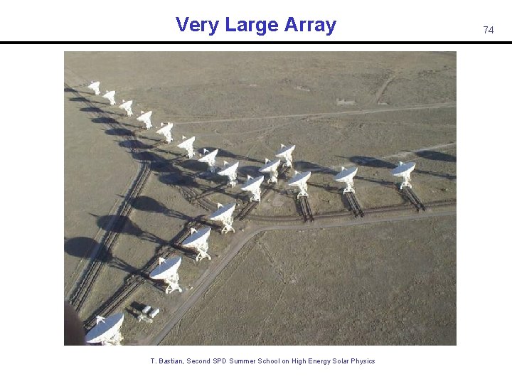
Very Large Array T. Bastian, Second SPD Summer School on High Energy Solar Physics 74

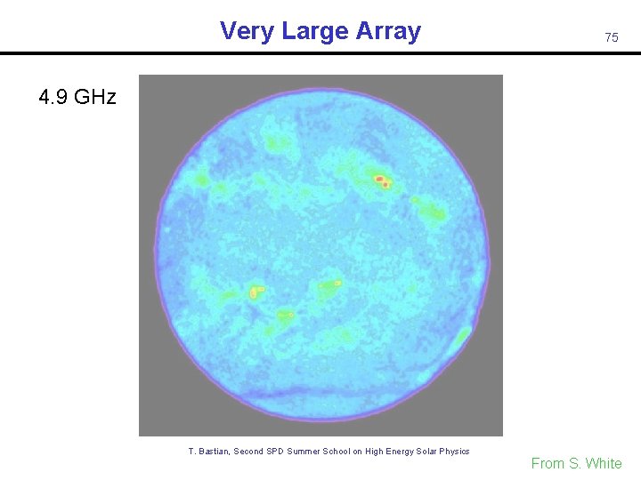
Very Large Array 75 4. 9 GHz T. Bastian, Second SPD Summer School on High Energy Solar Physics From S. White

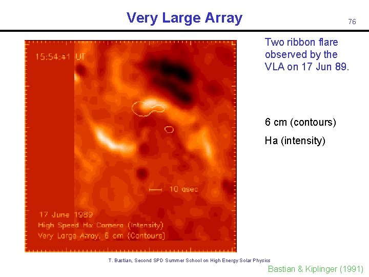
Very Large Array 76 Two ribbon flare observed by the VLA on 17 Jun 89. 6 cm (contours) Ha (intensity) T. Bastian, Second SPD Summer School on High Energy Solar Physics Bastian & Kiplinger (1991)

Nobeyama Radioheliograph T. Bastian, Second SPD Summer School on High Energy Solar Physics 77

Solar Radio Observations 17 GHz T. Bastian, Second SPD Summer School on High Energy Solar Physics 78

Nobeyama Radioheliograph T. Bastian, Second SPD Summer School on High Energy Solar Physics 79 From. S. S. White

Nobeyama Radioheliograph 17 GHz intensity 17 GHz circ. pol. 34 GHz intensity Time sequence of snapshot maps and 17 and 34 GHz. T. Bastian, Second SPD Summer School on High Energy Solar Physics 80

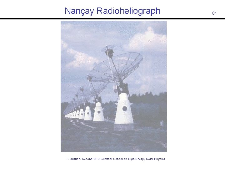
Nançay Radioheliograph T. Bastian, Second SPD Summer School on High Energy Solar Physics 81

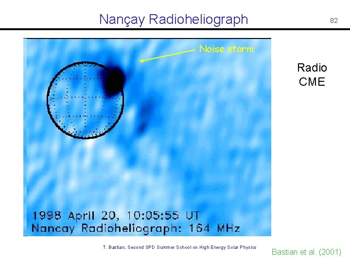
Nançay Radioheliograph 82 Noise storm Radio CME T. Bastian, Second SPD Summer School on High Energy Solar Physics Bastian et al. (2001)

83 T. Bastian, Second SPD Summer School on High Energy Solar Physics

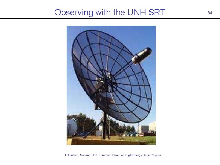
Observing with the UNH SRT T. Bastian, Second SPD Summer School on High Energy Solar Physics 84

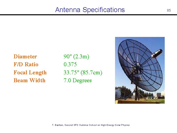
Antenna Specifications Diameter F/D Ratio Focal Length Beam Width 90" (2. 3 m) 0. 375 33. 75" (85. 7 cm) 7. 0 Degrees 85 T. Bastian, Second SPD Summer School on High Energy Solar Physics

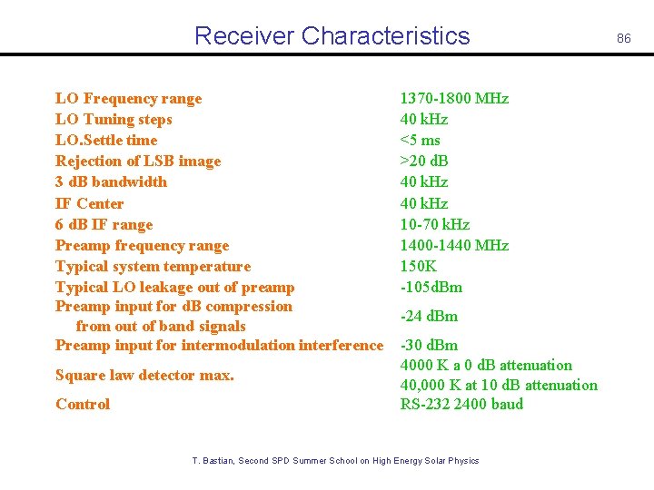
Receiver Characteristics LO Frequency range LO Tuning steps LO. Settle time Rejection of LSB image 3 d. B bandwidth IF Center 6 d. B IF range Preamp frequency range Typical system temperature Typical LO leakage out of preamp Preamp input for d. B compression from out of band signals Preamp input for intermodulation interference Square law detector max. Control 1370 -1800 MHz 40 k. Hz <5 ms >20 d. B 40 k. Hz 10 -70 k. Hz 1400 -1440 MHz 150 K -105 d. Bm -24 d. Bm -30 d. Bm 4000 K a 0 d. B attenuation 40, 000 K at 10 d. B attenuation RS-232 2400 baud T. Bastian, Second SPD Summer School on High Energy Solar Physics 86

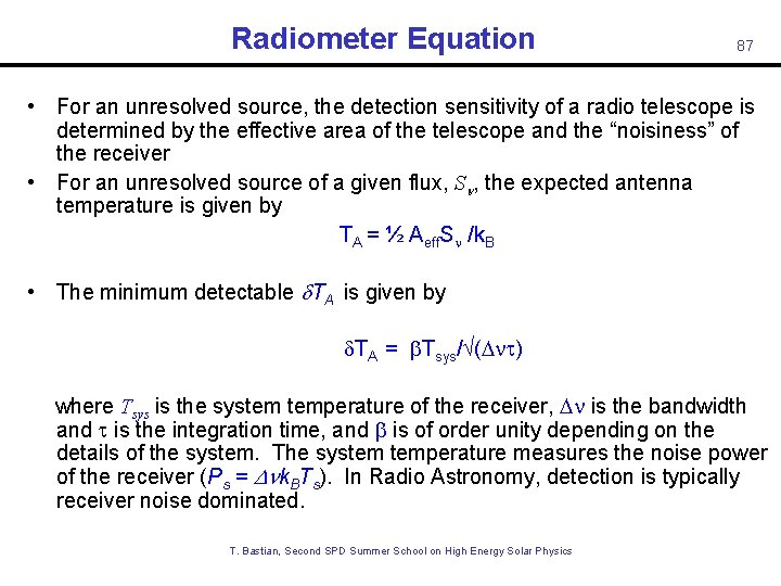
Radiometer Equation 87 • For an unresolved source, the detection sensitivity of a radio telescope is determined by the effective area of the telescope and the “noisiness” of the receiver • For an unresolved source of a given flux, S , the expected antenna temperature is given by TA = ½ Aeff. S /k. B • The minimum detectable TA is given by TA = Tsys/ (D ) where Tsys is the system temperature of the receiver, D is the bandwidth and is the integration time, and is of order unity depending on the details of the system. The system temperature measures the noise power of the receiver (Ps = D k. BTs). In Radio Astronomy, detection is typically receiver noise dominated. T. Bastian, Second SPD Summer School on High Energy Solar Physics

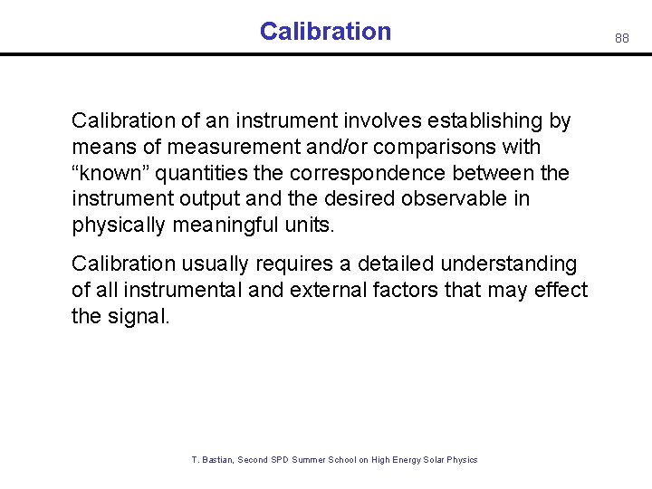
Calibration of an instrument involves establishing by means of measurement and/or comparisons with “known” quantities the correspondence between the instrument output and the desired observable in physically meaningful units. Calibration usually requires a detailed understanding of all instrumental and external factors that may effect the signal. T. Bastian, Second SPD Summer School on High Energy Solar Physics 88

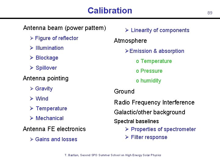
Calibration • Antenna beam (power pattern) Ø Figure of reflector Ø Illumination 89 Ø Linearity of components Atmosphere ØEmission & absorption Ø Blockage o Temperature Ø Spillover o Pressure • Antenna pointing Ø Gravity o humidity Ground Ø Wind Ø Temperature Ø Mechanical • Antenna FE electronics Ø Gains and losses Radio Frequency Interference Galactic/other background Spectral baselines Ø Properties of spectrometer Ø Filter response T. Bastian, Second SPD Summer School on High Energy Solar Physics

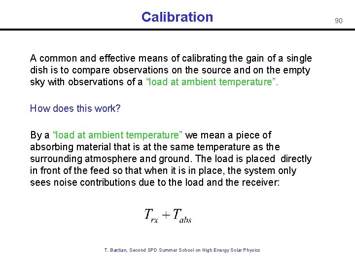
Calibration A common and effective means of calibrating the gain of a single dish is to compare observations on the source and on the empty sky with observations of a “load at ambient temperature”. How does this work? By a “load at ambient temperature” we mean a piece of absorbing material that is at the same temperature as the surrounding atmosphere and ground. The load is placed directly in front of the feed so that when it is in place, the system only sees noise contributions due to the load and the receiver: T. Bastian, Second SPD Summer School on High Energy Solar Physics 90

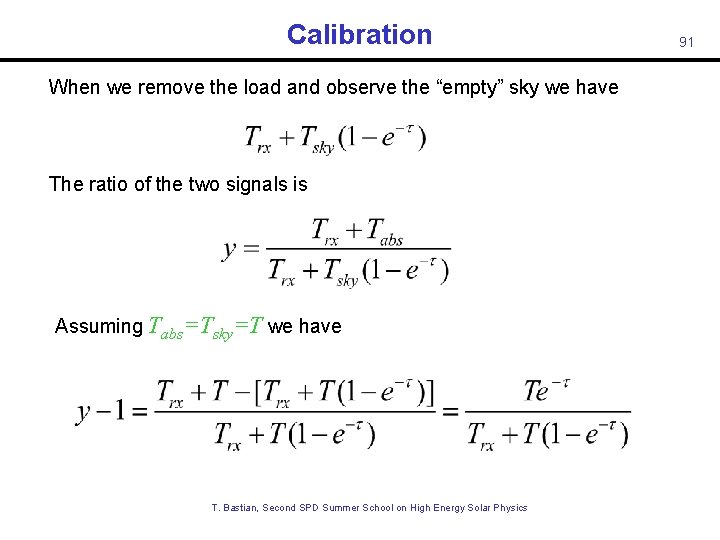
Calibration When we remove the load and observe the “empty” sky we have The ratio of the two signals is Assuming Tabs=Tsky=T we have T. Bastian, Second SPD Summer School on High Energy Solar Physics 91

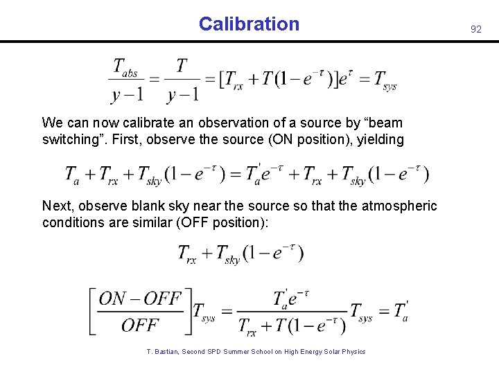
Calibration and We can now calibrate an observation of a source by “beam switching”. First, observe the source (ON position), yielding Next, observe blank sky near the source so that the atmospheric conditions are similar (OFF position): Then T. Bastian, Second SPD Summer School on High Energy Solar Physics 92

93 T. Bastian, Second SPD Summer School on High Energy Solar Physics

94 T. Bastian, Second SPD Summer School on High Energy Solar Physics

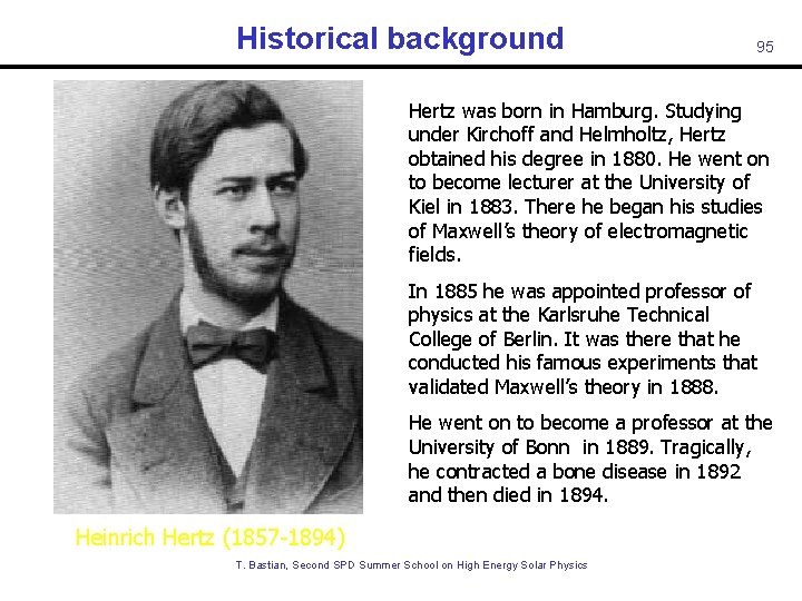
Historical background 95 Hertz was born in Hamburg. Studying under Kirchoff and Helmholtz, Hertz obtained his degree in 1880. He went on to become lecturer at the University of Kiel in 1883. There he began his studies of Maxwell’s theory of electromagnetic fields. In 1885 he was appointed professor of physics at the Karlsruhe Technical College of Berlin. It was there that he conducted his famous experiments that validated Maxwell’s theory in 1888. He went on to become a professor at the University of Bonn in 1889. Tragically, he contracted a bone disease in 1892 and then died in 1894. Heinrich Hertz (1857 -1894) T. Bastian, Second SPD Summer School on High Energy Solar Physics

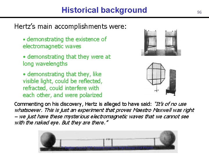
Historical background Hertz’s main accomplishments were: • demonstrating the existence of electromagnetic waves • demonstrating that they were at long wavelengths • demonstrating that they, like visible light, could be reflected, refracted, could interfere with each other, and were polarized Commenting on his discovery, Hertz is alleged to have said: “It’s of no use whatsoever. This is just an experiment that proves Maestro Maxwell was right – we just have these mysterious electromagnetic waves that we cannot see with the naked eye. But they are there. ” T. Bastian, Second SPD Summer School on High Energy Solar Physics 96

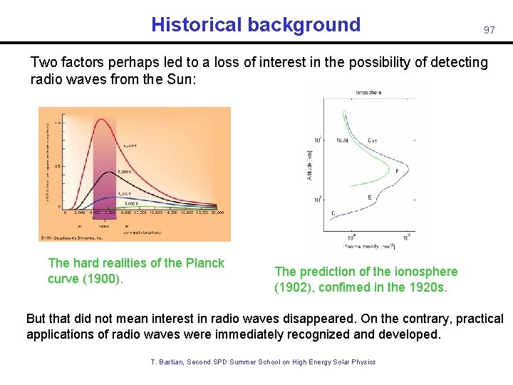
Historical background 97 Two factors perhaps led to a loss of interest in the possibility of detecting radio waves from the Sun: The hard realities of the Planck curve (1900). The prediction of the ionosphere (1902), confimed in the 1920 s. But that did not mean interest in radio waves disappeared. On the contrary, practical applications of radio waves were immediately recognized and developed. T. Bastian, Second SPD Summer School on High Energy Solar Physics

Historical background While Hertz may not have been seen further possibilities for his “Hertzian waves”, others saw both scientific and commercial possibilities: Scientific interest focused on the Sun: Thomas Edison suggested in 1890 that the Sun might be detectable at long wavelengths and proposed an experiment to do so. Sir Oliver Lodge actually tried to detect the Sun in 1894, but was unsuccessful. Johannes Wilsing and Julius Scheiner were the first to actually attempt detection of the Sun and to formally write up their results for a scientific journal in 1896. Charles Nordman also attempted to detect the Sun from high on Mont Blanc in 1900. In retrospect, this attempt should have been successful, but: solar minimum! T. Bastian, Second SPD Summer School on High Energy Solar Physics 98

Historical background Guglielmo Marconi (1874 -1937) T. Bastian, Second SPD Summer School on High Energy Solar Physics 99

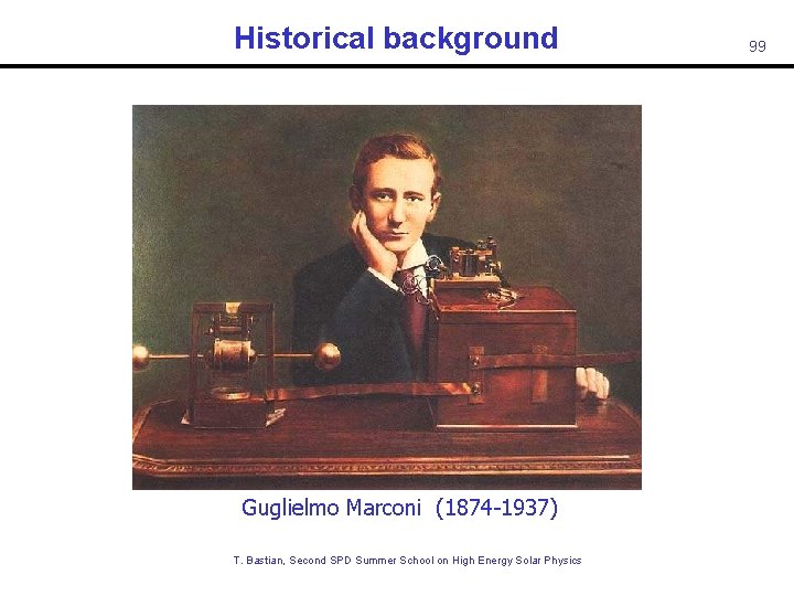
Historical background 100 Marconi was born in Bologna in 1874, the product of a wealthy Italian landowner, Giuseppe Marconi, and Annie Jameson (of Jameson Irish Whiskey! ). Marconi learned of Hertz’s groundbreaking experimental work at the time of Hertz’s death in 1894. He immediately thought of the possibility of using electromagnetic waves to transmit signals. He began experimenting with wireless transmission of signals and, in 1896, filed patents for the first wireless telegraphy system and founded the Wireless Telegraph & Signal Company in 1897. [Note: Lodge was actually the first to transmit wireless telegraphy, but considered it merely an academic exercise. ] The next few years saw rapid technical innovation that greatly increased the range of wireless communication. Marconi became the first to perform a wireless transmission and detection across the Atlantic Ocean in 1901. Wireless grew in leaps and bounds thereafter making Marconi and his company rich and influential. T. Bastian, Second SPD Summer School on High Energy Solar Physics

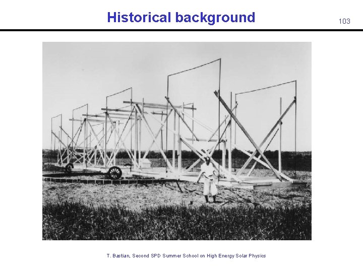
Historical background 101 It was not until the 1930 s that scientific interest in radio waves was renewed, and only because a young engineer with Bell Telephone was tasked with investigating sources of noise in transatlantic radio communications. Karl Jansky (1905 -1950) built an antenna that operated at 14 m and, after making observations for several months, identified two types of noise: • Local and more distant thunderstorms • A faint, steady hiss of unknown origin Further work showed that the latter did not repeat every 24 h, as might be expected for a terrestrial source, but every 23 h 56 m! Jansky demonstrated that the source of the noise was toward Sagittarius, the center of the Milky Way. His results were reported in the New York Times in May, 1933. While Jansky wanted to continue his investigations, Bell Lab had its answer and moved him to other pursuits. He never returned to radio astronomy. Nevertheless, the fundamental unit of radio flux bears his name: 1 Jansky = 10 -26 Watts m-2 Hz-1 T. Bastian, Second SPD Summer School on High Energy Solar Physics

Historical background The Sun was finally detected during WW II. Both J. S. Hey and, independently, G. Southworth (1942) discovered radio emission from the Sun as part of their investigations of potential jamming of radar stations by the Germans. Their discoveries were suppressed until after the war for security reasons. WW II played a major role in finally jumpstarting radio astronomy as an independent scientific discipline. The war resulted in a great many radio and radar engineers. Stimulated by discoveries by Jansky, Reber, Southworth, and Hey – coupled with the availability of trained personnel - radio astronomy leaped forward after the War. T. Bastian, Second SPD Summer School on High Energy Solar Physics 102

Historical background T. Bastian, Second SPD Summer School on High Energy Solar Physics 103

104 T. Bastian, Second SPD Summer School on High Energy Solar Physics