1 Overview Suffix tries Online construction of suffix

1

Overview · Suffix tries · On-line construction of suffix tries in quadratic time · Suffix trees · On-line construction of suffix trees in linear time · Applications 2

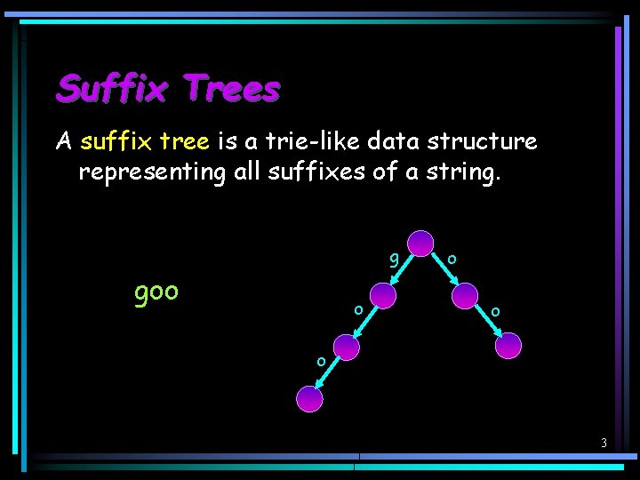
Suffix Trees A suffix tree is a trie-like data structure representing all suffixes of a string. g goo o o 3

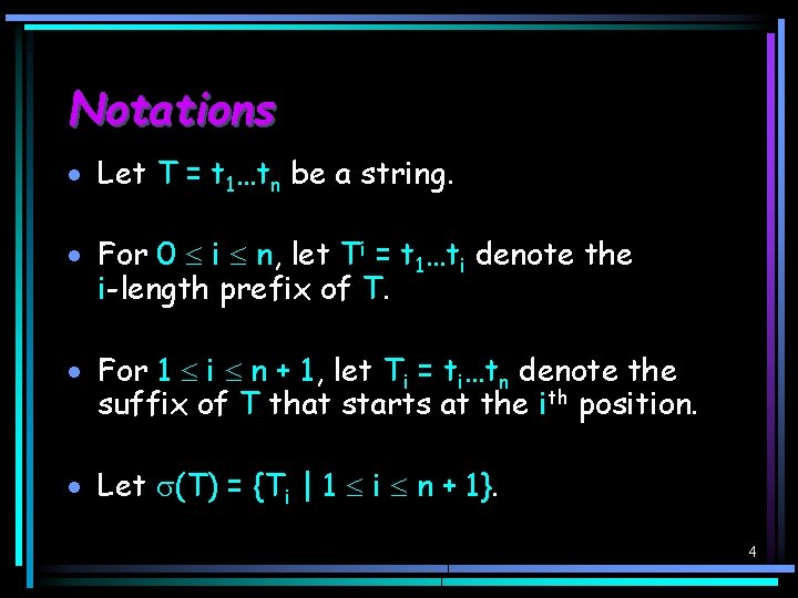
Notations · Let T = t 1…tn be a string. · For 0 i n, let Ti = t 1…ti denote the i-length prefix of T. · For 1 i n + 1, let Ti = ti…tn denote the suffix of T that starts at the ith position. · Let (T) = {Ti | 1 i n + 1}. 4

Suffix Tries The suffix trie of T, denoted by STrie(T), is a trie representing (T). 5

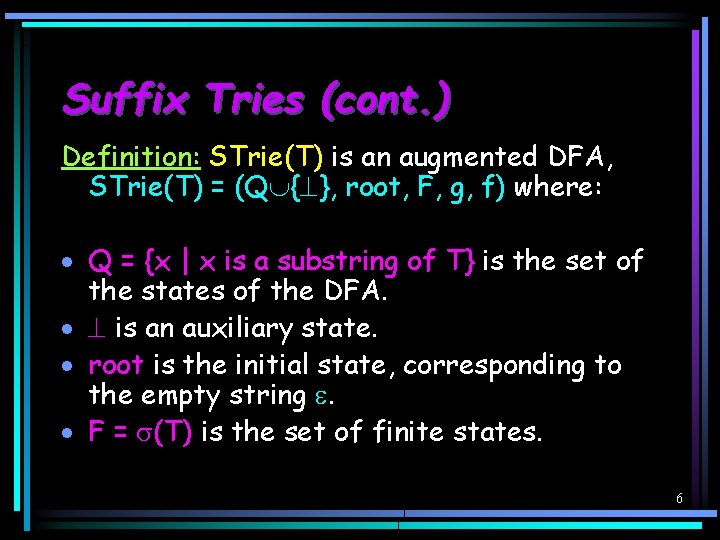
Suffix Tries (cont. ) Definition: STrie(T) is an augmented DFA, STrie(T) = (Q { }, root, F, g, f) where: · Q = {x | x is a substring of T} is the set of the states of the DFA. · is an auxiliary state. · root is the initial state, corresponding to the empty string . · F = (T) is the set of finite states. 6

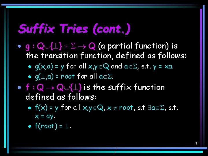
Suffix Tries (cont. ) · g : Q { } Q (a partial function) is the transition function, defined as follows: · g(x, a) = y for all x, y Q and a , s. t. y = xa. · g( , a) = root for all a . · f : Q Q { } is the suffix function defined as follows: · f(x) = y for all x, y Q, x root, s. t a , s. t. x = ay. · f(root) = . 7

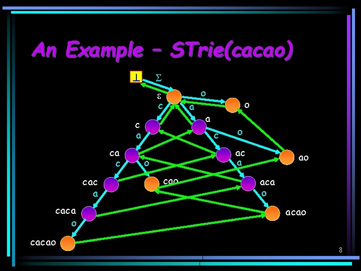
An Example – STrie(cacao) c c a ca c cac a caca o cacao a o o a c o ac a o cao ao acao 8

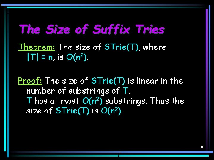
The Size of Suffix Tries Theorem: The size of STrie(T), where |T| = n, is O(n 2). Proof: The size of STrie(T) is linear in the number of substrings of T. T has at most O(n 2) substrings. Thus the size of STrie(T) is O(n 2). 9

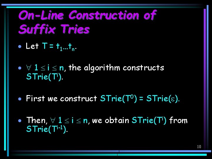
On-Line Construction of Suffix Tries · Let T = t 1…tn. · 1 i n, the algorithm constructs STrie(Ti). · First we construct STrie(T 0) = STrie( ). · Then, 1 i n, we obtain STrie(Ti) from STrie(Ti-1). 10

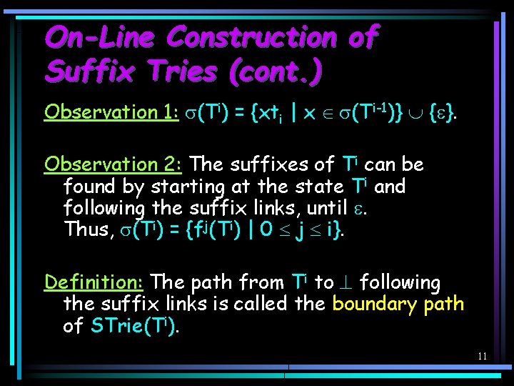
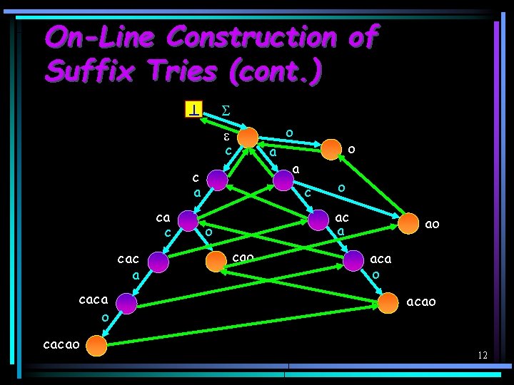
On-Line Construction of Suffix Tries (cont. ) Observation 1: (Ti) = {xti | x (Ti-1)} { }. Observation 2: The suffixes of Ti can be found by starting at the state Ti and following the suffix links, until . Thus, (Ti) = {fj(Ti) | 0 j i}. Definition: The path from Ti to following the suffix links is called the boundary path of STrie(Ti). 11

On-Line Construction of Suffix Tries (cont. ) c c a ca c cac a caca o cacao a o o a c o ac a o cao ao acao 12

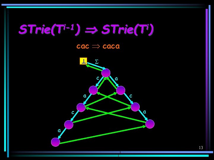
STrie(Ti-1) STrie(Ti) caca c a c a a 13

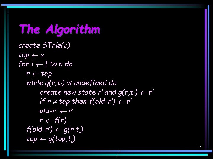
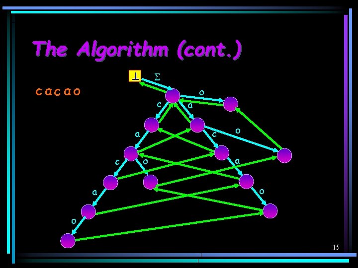
The Algorithm create STrie( ) top for i 1 to n do r top while g(r, ti) is undefined do create new state r’ and g(r, ti) r’ if r top then f(old-r’) r’ old-r’ r’ r f(r) f(old-r’) g(r, ti) top g(top, ti) 14

The Algorithm (cont. ) cac ao c a a o c o o a o o 15

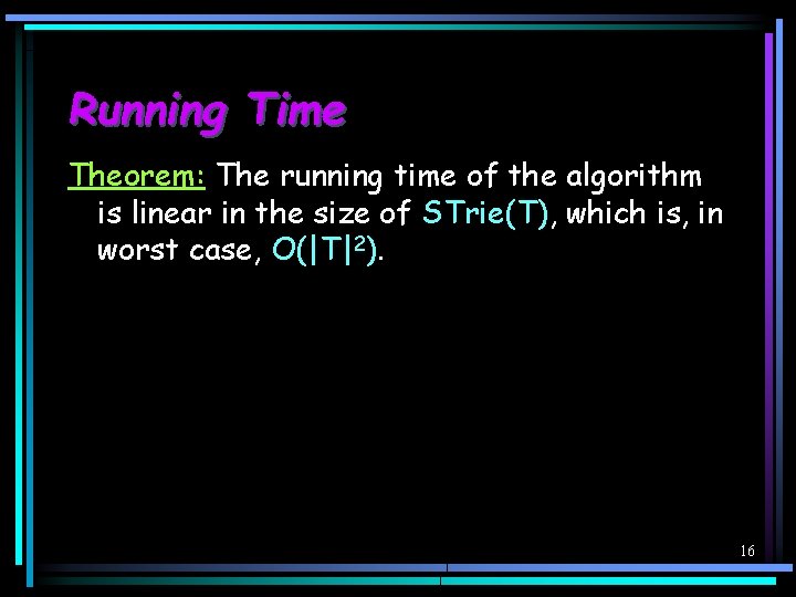
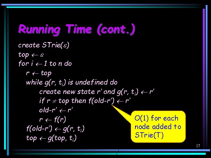
Running Time Theorem: The running time of the algorithm is linear in the size of STrie(T), which is, in worst case, O(|T|2). 16

Running Time (cont. ) create STrie( ) top for i 1 to n do r top while g(r, ti) is undefined do create new state r’ and g(r, ti) r’ if r top then f(old-r’) r’ old-r’ r’ O(1) for each r f(r) node added to f(old-r’) g(r, ti) STrie(T) top g(top, ti) 17

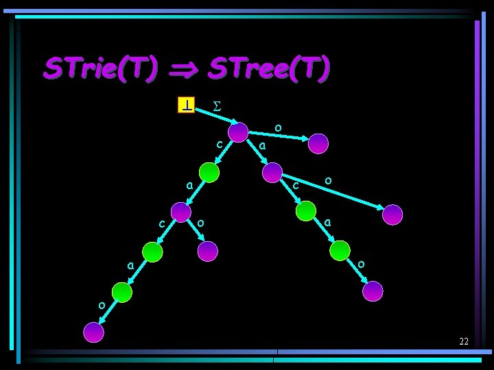
Suffix Trees · A suffix tree STree(T) represents STrie(T) in space linear in |T|. · This is achieved by representing only a subset of Q’ { } of Q { }, called the explicit states. 18

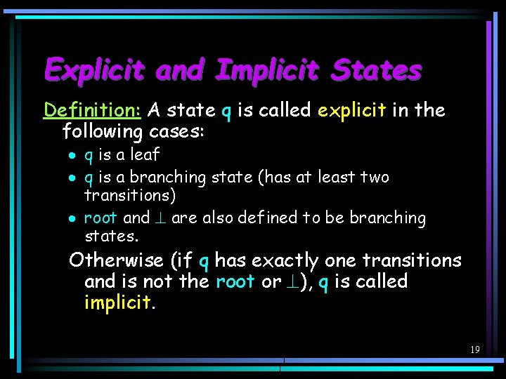
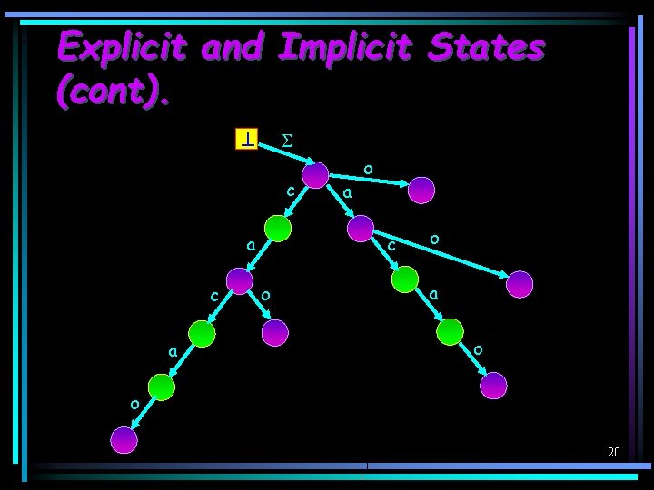
Explicit and Implicit States Definition: A state q is called explicit in the following cases: · q is a leaf · q is a branching state (has at least two transitions) · root and are also defined to be branching states. Otherwise (if q has exactly one transitions and is not the root or ), q is called implicit. 19

Explicit and Implicit States (cont). c a a o c o o a o o 20

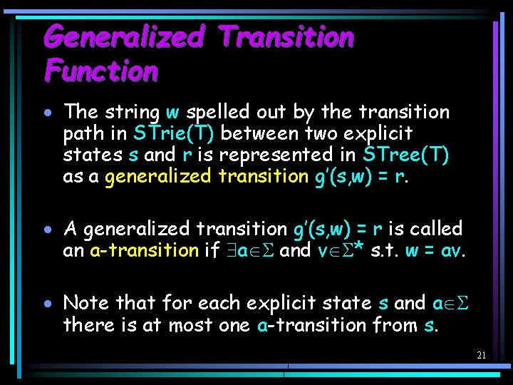
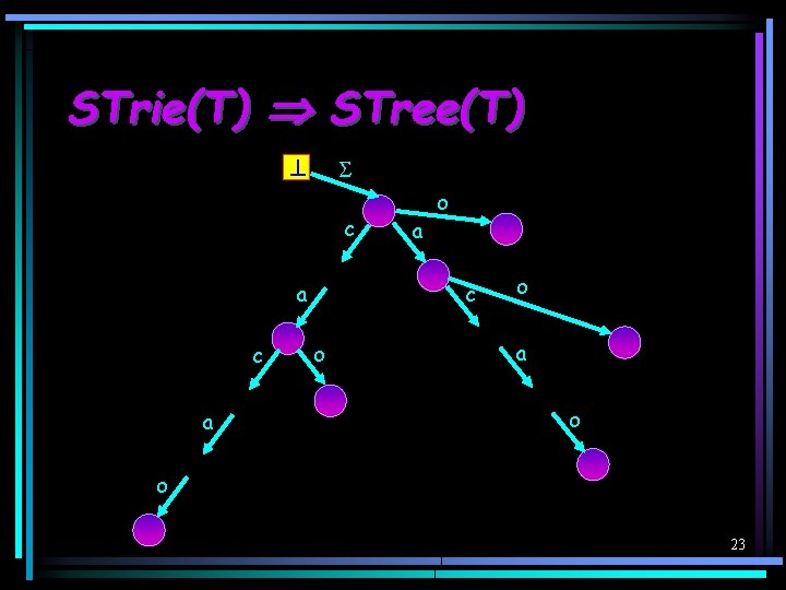
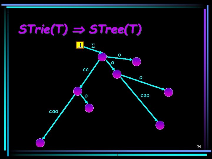
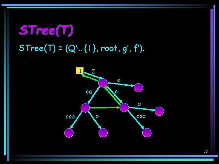
Generalized Transition Function · The string w spelled out by the transition path in STrie(T) between two explicit states s and r is represented in STree(T) as a generalized transition g’(s, w) = r. · A generalized transition g’(s, w) = r is called an a-transition if a and v * s. t. w = av. · Note that for each explicit state s and a there is at most one a-transition from s. 21

STrie(T) STree(T) c a a o c o o a o o 22

STrie(T) STree(T) c a a o c o o a o o 23

STrie(T) STree(T) ca o o cao 24

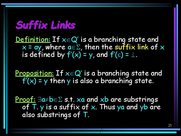
Suffix Links Definition: If x Q’ is a branching state and x = ay, where a , then the suffix link of x is defined by f’(x) = y, and f’( ) = . Proposition: If x Q’ is a branching state and f’(x) = y then y is also a branching state. Proof: a b s. t. xa and xb are substrings of T. y is a suffix of x. Thus ya and yb are also substrings of T. 25

STree(T) = (Q’ { }, root, g’, f’). o a ca o cao 26

The Size of Suffix Trees Theorem: The size of STree(T), where |T| = n, is O(n). Proof: Since we represent each substring w = tk…tp of T by a pair pointers (k, p), the size of STree(T) is linear in the number of explicit states. STree(T) has at most n leaves, and thus at most n - 1 branching states. Therefore, the size of STree(T) is O(n). 27

Reference Pairs Definition: Let r be an explicit or implicit state. (s, w) is called a reference pair for r if: · · s is an explicit state and an ancestor of r. w is the string spelled out by the transitions from s to r in the corresponding suffix trie. Definition: A reference pair (s, w) for r is called canonical if s is the closest explicit ancestor of r (or r itself, if it is explicit). 28

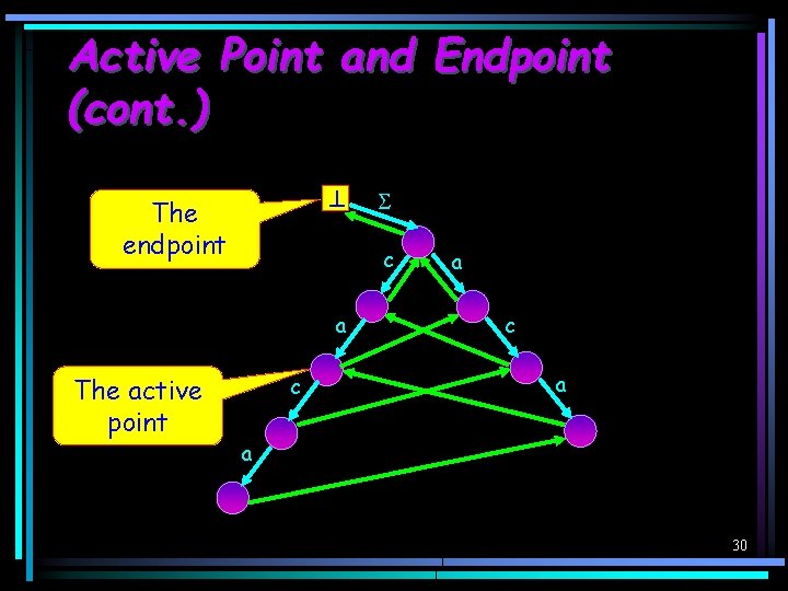
Active Point and Endpoint Let s 1 = Ti-1, s 2, …, si = root, si+1 = be the boundary path of STrie(Ti-1). Definition: sj is called the active point of STrie(Ti-1) if j is the smallest index for which sj is not a leaf. Definition: sj’ is called the endpoint of STrie(Ti-1) if j’ is the smallest index for which g(sj’, ti) is defined. 29

Active Point and Endpoint (cont. ) The endpoint c a The active point c a a 30

Active Point and Endpoint (cont. ) Proposition: sj and sj’ are well defined and j j’. Proof: · root is not a leaf sj is defined. · g( , ti) is defined sj’ is defined. · g(sj’, ti) is defined sj’ is not a leaf j j’. 31

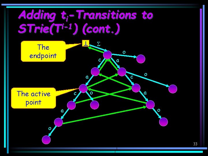
Adding ti-Transitions to STrie(Ti-1) Lemma: When obtaining STrie(Ti) from STrie(Ti-1) the algorithm adds a ti-transition to each state sh s. t. 1 h < j’, and only to these states, as follows: · For 1 h < j, the new transition expands an old branch of the trie that ends at s h. · For j h < j’, the new transition initiates a new branch from sh. 32

Adding ti-Transitions to STrie(Ti-1) (cont. ) The endpoint c a The active point c a o a c o o a o o 33

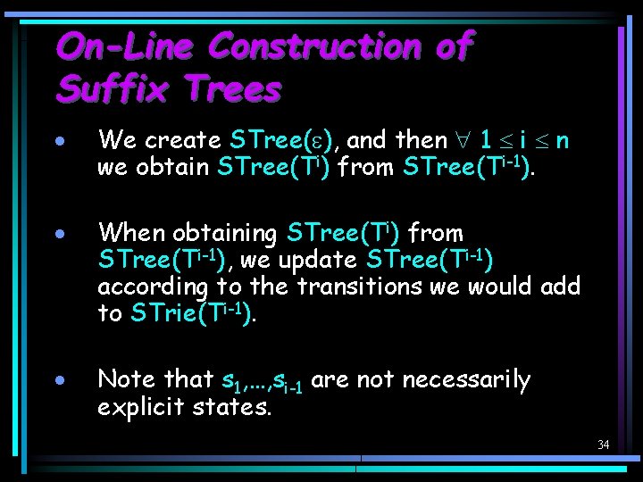
On-Line Construction of Suffix Trees · We create STree( ), and then 1 i n we obtain STree(Ti) from STree(Ti-1). · When obtaining STree(Ti) from STree(Ti-1), we update STree(Ti-1) according to the transitions we would add to STrie(Ti-1). · Note that s 1, …, si-1 are not necessarily explicit states. 34

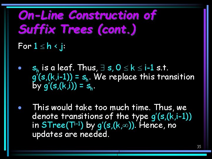
On-Line Construction of Suffix Trees (cont. ) For 1 h < j: · sh is a leaf. Thus, s, 0 k i-1 s. t. g’(s, (k, i-1)) = sh. We replace this transition by g’(s, (k, i)) = sh. · This would take too much time. Thus, we denote transitions of the type g’(s, (k, i-1)) in STree(Ti-1) by g’(s, (k, )). Hence, no updates are needed. 35

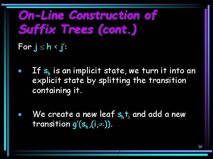
On-Line Construction of Suffix Trees (cont. ) For j h < j’: · If sh is an implicit state, we turn it into an explicit state by splitting the transition containing it. · We create a new leaf shti and add a new transition g’(sh, (i, )). 36

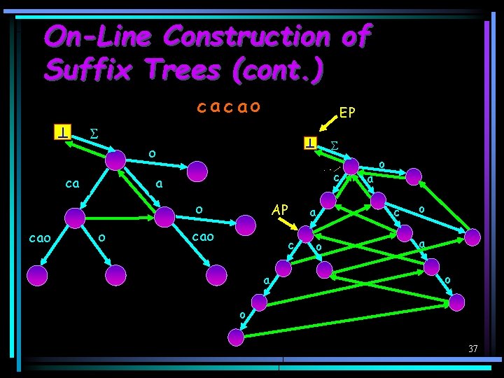
On-Line Construction of Suffix Trees (cont. ) cac ao EP o cac ca cacao caca cac EPAP aaca acao aac o cao o AP cao c a EP c a o c o a o o 37

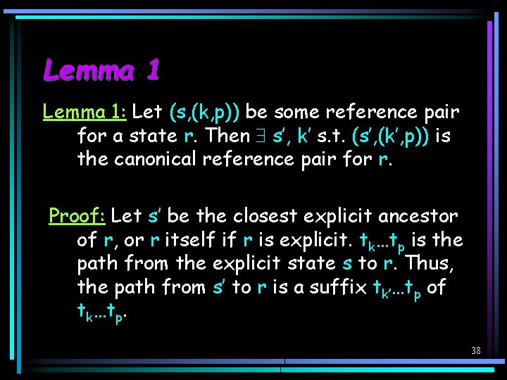
Lemma 1: Let (s, (k, p)) be some reference pair for a state r. Then s’, k’ s. t. (s’, (k’, p)) is the canonical reference pair for r. Proof: Let s’ be the closest explicit ancestor of r, or r itself if r is explicit. tk…tp is the path from the explicit state s to r. Thus, the path from s’ to r is a suffix tk’…tp of tk…tp. 38

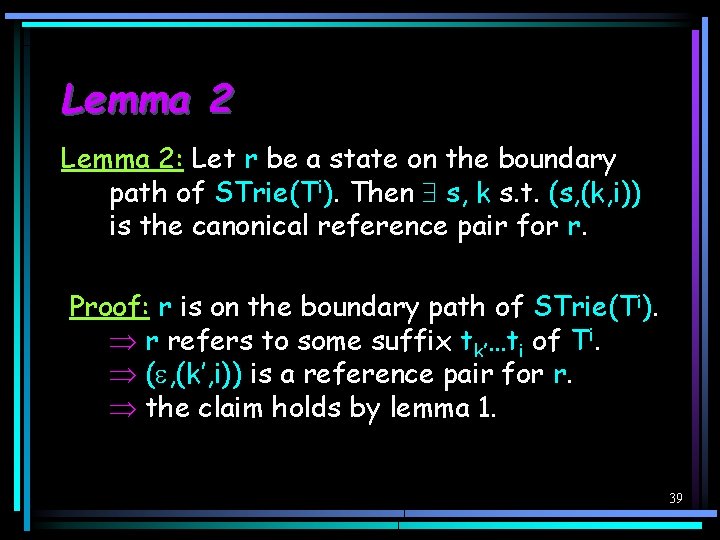
Lemma 2: Let r be a state on the boundary path of STrie(Ti). Then s, k s. t. (s, (k, i)) is the canonical reference pair for r. Proof: r is on the boundary path of STrie(Ti). r refers to some suffix tk’…ti of Ti. ( , (k’, i)) is a reference pair for r. the claim holds by lemma 1. 39

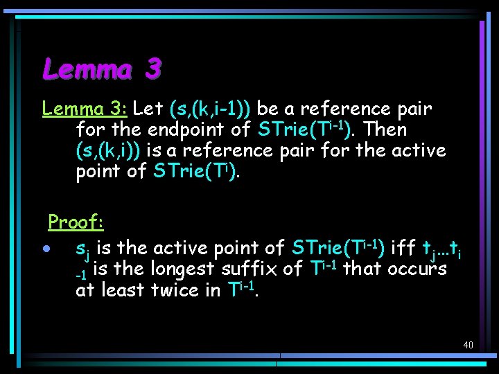
Lemma 3: Let (s, (k, i-1)) be a reference pair for the endpoint of STrie(Ti-1). Then (s, (k, i)) is a reference pair for the active point of STrie(Ti). Proof: · sj is the active point of STrie(Ti-1) iff tj…ti i-1 that occurs is the longest suffix of T -1 at least twice in Ti-1. 40

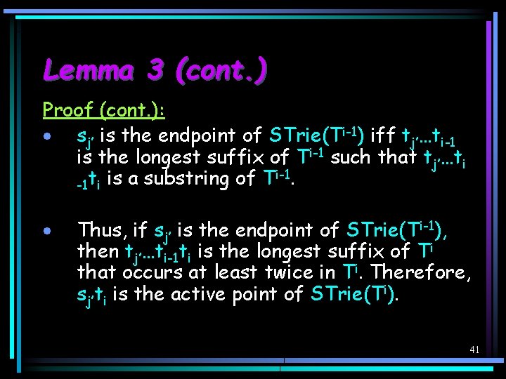
Lemma 3 (cont. ) Proof (cont. ): · sj’ is the endpoint of STrie(Ti-1) iff tj’…ti-1 is the longest suffix of Ti-1 such that tj’…ti i-1. t is a substring of T -1 i · Thus, if sj’ is the endpoint of STrie(Ti-1), then tj’…ti-1 ti is the longest suffix of Ti that occurs at least twice in Ti. Therefore, sj’ti is the active point of STrie(Ti). 41

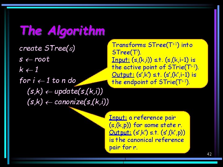
The Algorithm create STree( ) s root k 1 for i 1 to n do (s, k) update(s, (k, i)) (s, k) canonize(s, (k, i)) Transforms STree(Ti-1) into STree(Ti). Input: (s, (k, i)) s. t. (s, (k, i-1) is the active point of STrie(Ti-1). Output: (s’, k’) s. t. (s’, (k’, i-1) is the endpoint of STrie(Ti-1). Input: a reference pair (s, (k, p)) for some state r. Output: (s’, k’) s. t. (s’, (k’, p)) is the canonical reference pair for r. 42

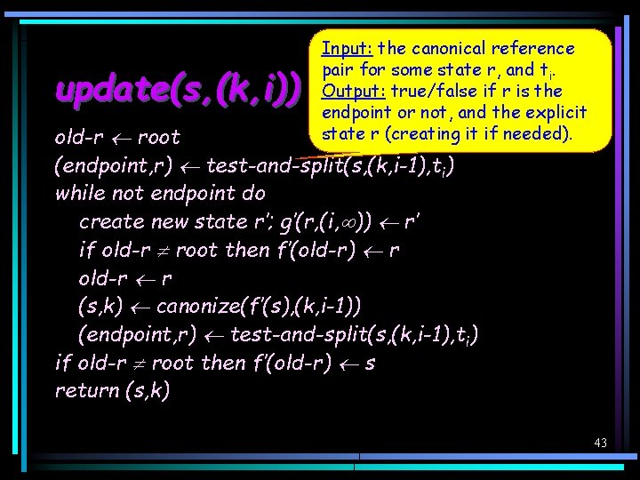
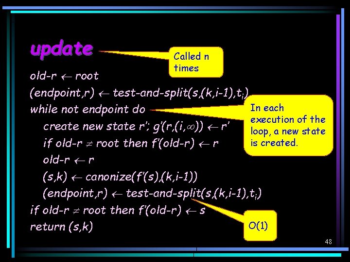
update(s, (k, i)) Input: the canonical reference pair for some state r, and ti. Output: true/false if r is the endpoint or not, and the explicit state r (creating it if needed). old-r root (endpoint, r) test-and-split(s, (k, i-1), ti) while not endpoint do create new state r’; g’(r, (i, )) r’ if old-r root then f’(old-r) r old-r r (s, k) canonize(f’(s), (k, i-1)) (endpoint, r) test-and-split(s, (k, i-1), ti) if old-r root then f’(old-r) s return (s, k) 43

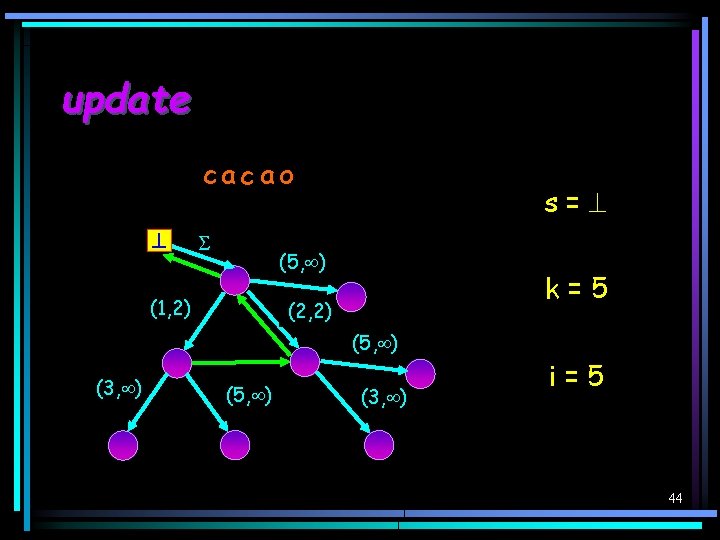
update cac ao s s= =root (5, ) (1, 2) k=2 3 4 5 1 (2, 2) (2, ) (5, ) (3, ) i=4 2 5 3 1 44

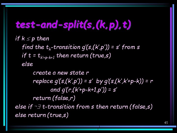
test-and-split(s, (k, p), t) if k p then find the tk-transition g’(s, (k’, p’)) = s’ from s if t = tk’+p-k+1 then return (true, s) else create a new state r replace g’(s, (k’, p’)) = s’ by g’(s, (k’, k’+p-k)) = r and g’(r, (k’+p-k+1, p’)) = s’ return (false, r) else if t-transition from s then return (false, s) else return (true, s) 45

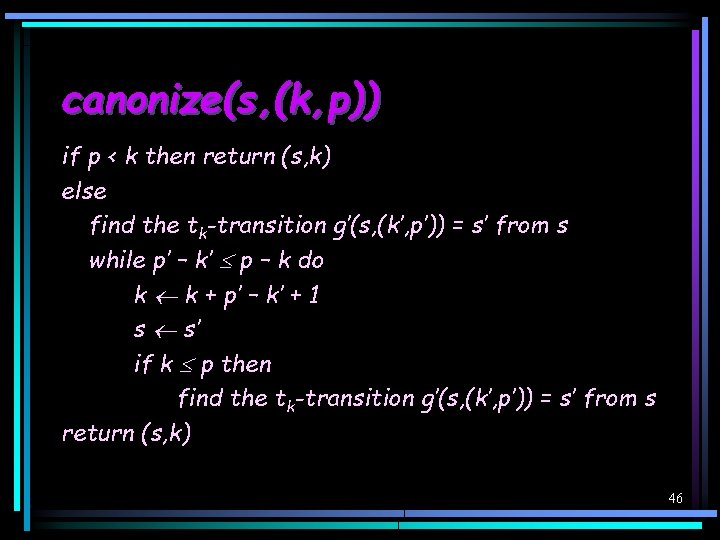
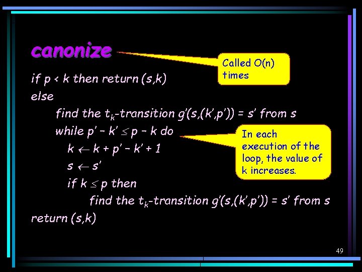
canonize(s, (k, p)) if p < k then return (s, k) else find the tk-transition g’(s, (k’, p’)) = s’ from s while p’ – k’ p – k do k k + p’ – k’ + 1 s s’ if k p then find the tk-transition g’(s, (k’, p’)) = s’ from s return (s, k) 46

Running Time Theorem: The running time of the algorithm is O(n). Proof: We divide the running time into two components: 1. The total time of the procedure canonize. 2. The rest. 47

update Called n times old-r root (endpoint, r) test-and-split(s, (k, i-1), ti) In each while not endpoint do execution of the create new state r’; g’(r, (i, )) r’ loop, a new state is created. if old-r root then f’(old-r) r old-r r (s, k) canonize(f’(s), (k, i-1)) (endpoint, r) test-and-split(s, (k, i-1), ti) if old-r root then f’(old-r) s O(1) return (s, k) 48

canonize Called O(n) times if p < k then return (s, k) else find the tk-transition g’(s, (k’, p’)) = s’ from s while p’ – k’ p – k do In each execution of the k k + p’ – k’ + 1 loop, the value of s s’ k increases. if k p then find the tk-transition g’(s, (k’, p’)) = s’ from s return (s, k) 49

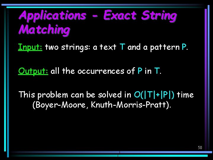
Applications - Exact String Matching Input: two strings: a text T and a pattern P. Output: all the occurrences of P in T. This problem can be solved in O(|T|+|P|) time (Boyer-Moore, Knuth-Morris-Pratt). 50

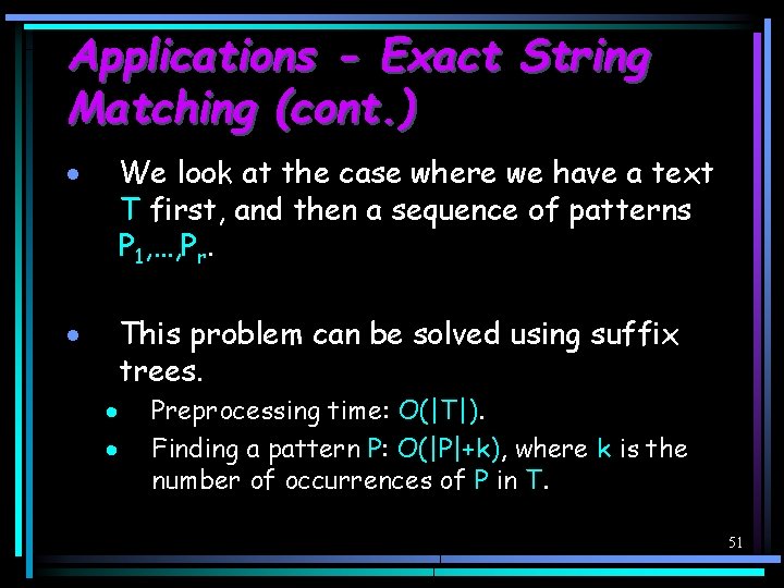
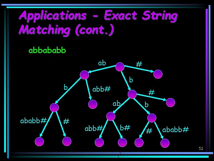
Applications - Exact String Matching (cont. ) · We look at the case where we have a text T first, and then a sequence of patterns P 1, …, Pr. · This problem can be solved using suffix trees. · · Preprocessing time: O(|T|). Finding a pattern P: O(|P|+k), where k is the number of occurrences of P in T. 51

Applications - Exact String Matching (cont. ) abbababb ab b # b abb# # ab ababb# # abb# b# b # ababb# 52

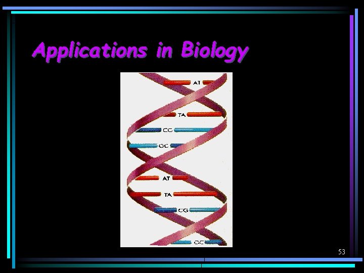
Applications in Biology 53

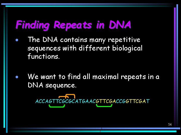
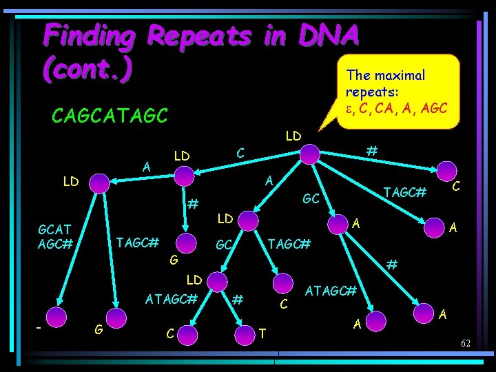
Finding Repeats in DNA · The DNA contains many repetitive sequences with different biological functions. · We want to find all maximal repeats in a DNA sequence. ACCAGTTCGCGCATGAACGTTCGACCGGTTCGAT 54

Finding Repeats in DNA (cont. ) Theorem: All maximal repeats in a sequence T can be found in O(|T|) time using suffix trees. 55

Finding Repeats in DNA (cont. ) Lemma: If w is a maximal repeat in T, then the state w in STree(T) is explicit. Proof: If w is a maximal repeat then there at least two occurrences of w in T s. t. the character following w is different. Thus w is a branching state, and therefore it is explicit. 56

Finding Repeats in DNA (cont. ) Corollary: There at most O(|T|) maximal repeats in T. Proof: By the above lemma, each maximal repeat corresponds to an explicit state. Since STree(T) has O(|T|) explicit states, T has O(|T|) maximal repeats. 57

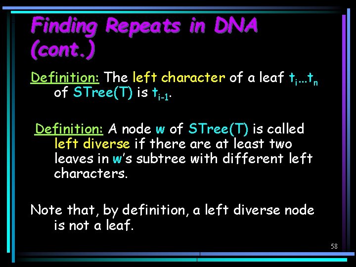
Finding Repeats in DNA (cont. ) Definition: The left character of a leaf ti…tn of STree(T) is ti-1. Definition: A node w of STree(T) is called left diverse if there at least two leaves in w’s subtree with different left characters. Note that, by definition, a left diverse node is not a leaf. 58

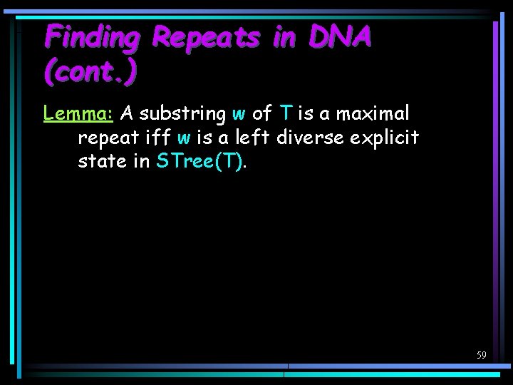
Finding Repeats in DNA (cont. ) Lemma: A substring w of T is a maximal repeat iff w is a left diverse explicit state in STree(T). 59

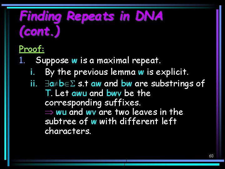
Finding Repeats in DNA (cont. ) Proof: 1. Suppose w is a maximal repeat. i. By the previous lemma w is explicit. ii. a b s. t aw and bw are substrings of T. Let awu and bwv be the corresponding suffixes. wu and wv are two leaves in the subtree of w with different left characters. 60

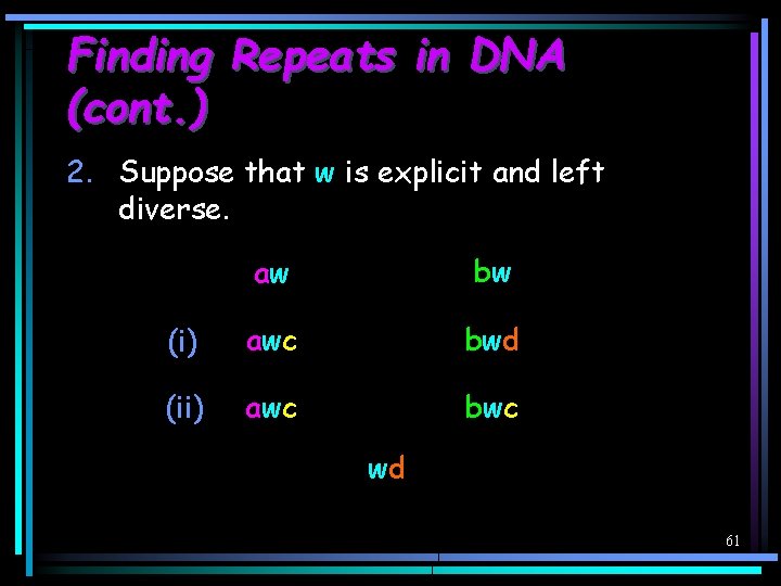
Finding Repeats in DNA (cont. ) 2. Suppose that w is explicit and left diverse. aw bw (i) awc bwd (ii) awc bwc wd 61

Finding Repeats in DNA (cont. ) The maximal repeats: , C, CA, A, AGC CAGCATAGC LD A # GCAT AGC# TAGC# LD A ATAGC# G C A TAGC# GC G C TAGC# GC # LD - # C LD # C T ATAGC# A A 62

Bibliography · On-Line Construction of Suffix Trees E. Ukkonen · Algorithms on String, Trees, and Sequences Dan Gusfield 63