1 Overview Some basic math l Error correcting

1

Overview Some basic math l Error correcting codes l Low degree polynomials l Introduction to consistent readers and consistency tests l H. W 2

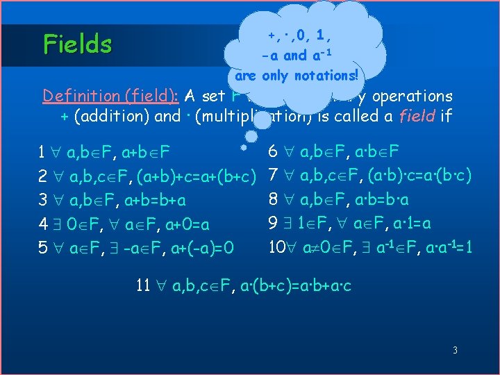
Fields +, ·, 0, 1, -a and a-1 are only notations! Definition (field): A set F with two binary operations + (addition) and · (multiplication) is called a field if 1 a, b F, a+b F 2 a, b, c F, (a+b)+c=a+(b+c) 3 a, b F, a+b=b+a 4 0 F, a F, a+0=a 5 a F, -a F, a+(-a)=0 6 a, b F, a·b F 7 a, b, c F, (a·b)·c=a·(b·c) 8 a, b F, a·b=b·a 9 1 F, a F, a· 1=a 10 a 0 F, a-1 F, a·a-1=1 11 a, b, c F, a·(b+c)=a·b+a·c 3

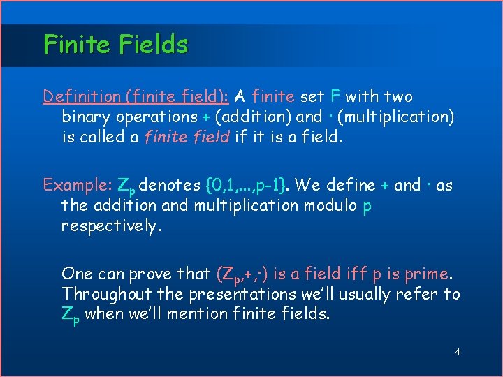
Finite Fields Definition (finite field): A finite set F with two binary operations + (addition) and · (multiplication) is called a finite field if it is a field. Example: Zp denotes {0, 1, . . . , p-1}. We define + and · as the addition and multiplication modulo p respectively. One can prove that (Zp, +, ·) is a field iff p is prime. Throughout the presentations we’ll usually refer to Zp when we’ll mention finite fields. 4

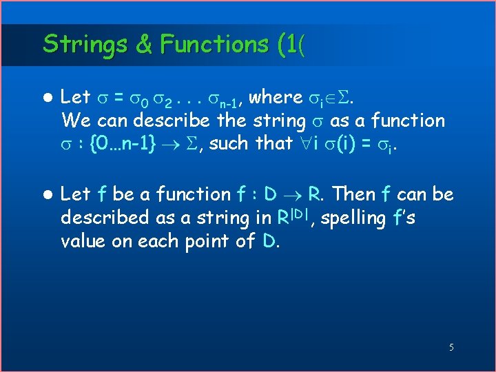
Strings & Functions (1( l Let = 0 2. . . n-1, where i . We can describe the string as a function : {0…n-1} , such that i (i) = i. l Let f be a function f : D R. Then f can be described as a string in R|D|, spelling f’s value on each point of D. 5

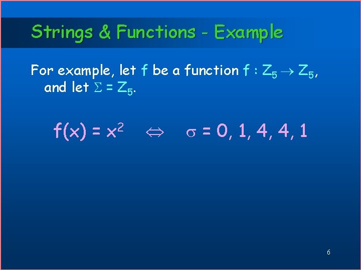
Strings & Functions - Example For example, let f be a function f : Z 5, and let = Z 5. f(x) = x 2 = 0, 1, 4, 4, 1 6

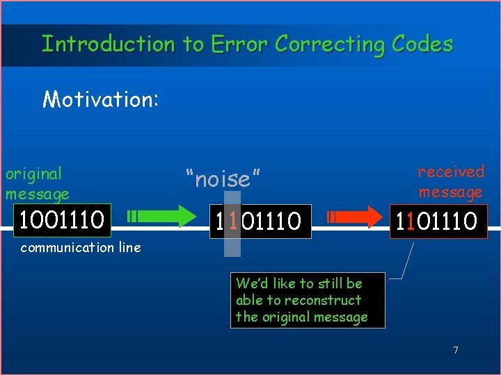
Introduction to Error Correcting Codes Motivation: original message 1001110 “noise” 1 1001110 received message 1101110 communication line We’d like to still be able to reconstruct the original message 7

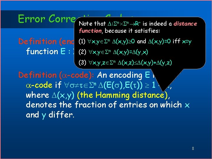
Error Correcting Codes Note that : R is indeed a distance function, because it satisfies: m m + m (x, y) 0 and (x, y)=0 iff x=y (1) x, y Definition (encoding): An encoding E is a m (x, y)= (y, x) function E : n(2) x, y m, where m >> n. (3) x, y, z m (x, z) (x, y)+ (y, z) Definition ( -code): An encoding E is an -code if n (E( ), E( )) 1 - , where (x, y) (the Hamming distance), denotes the fraction of entries on which x and y differ. 8

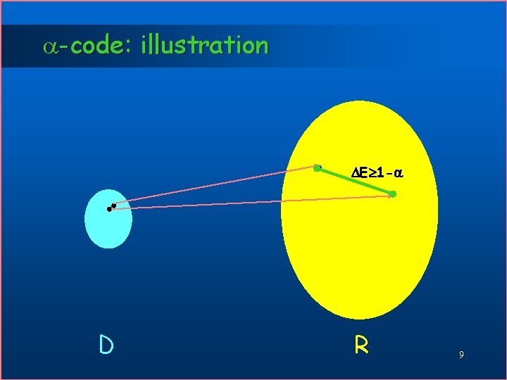
-code: illustration E 1 - D R 9

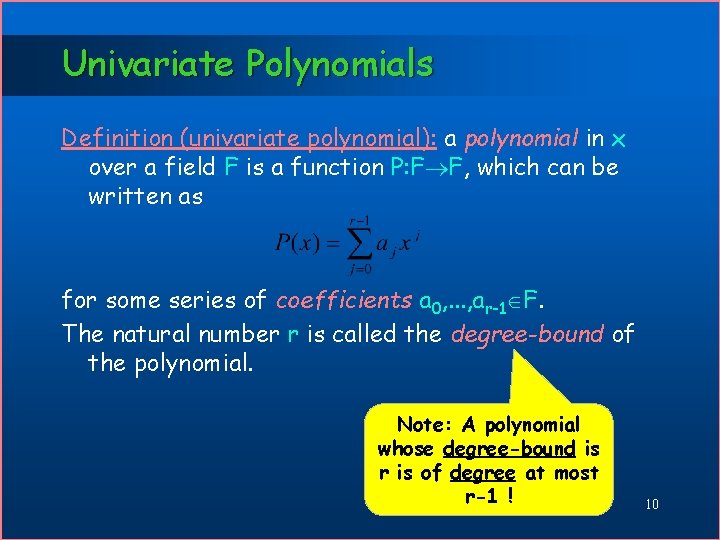
Univariate Polynomials Definition (univariate polynomial): a polynomial in x over a field F is a function P: F F, which can be written as for some series of coefficients a 0, . . . , ar-1 F. The natural number r is called the degree-bound of the polynomial. Note: A polynomial whose degree-bound is r is of degree at most r-1 ! 10

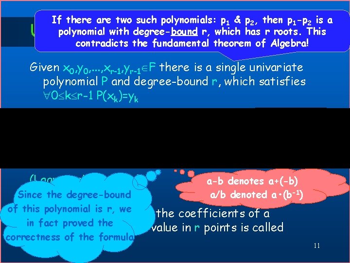
If there are two such polynomials: p 1 & p 2, then p 1 -p 2 is a polynomial with degree-bound r, which has r roots. This contradicts the fundamental theorem of Algebra! Univariate Interpolation Given x 0, y 0, . . . , xr-1, yr-1 F there is a single univariate polynomial P and degree-bound r, which satisfies 0 k r-1 P(xk)=yk yt 0 (Lagrange’s formula) a-b denotes a+(-b) a/b denoted a • (b-1) Since the degree-bound Let’s check the value of of this polynomial is r, we process the coefficients of a this. The polynomial in xof= finding xt in fact proved the polynomial for some 0 t given r-1: its value in r points is called correctness of the formula interpolation. 11

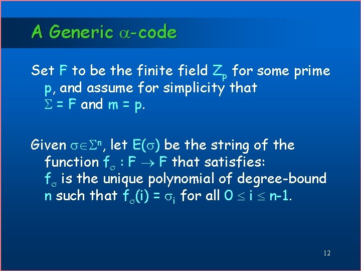
A Generic -code Set F to be the finite field Zp for some prime p, and assume for simplicity that = F and m = p. Given n, let E( ) be the string of the function f : F F that satisfies: f is the unique polynomial of degree-bound n such that f (i) = i for all 0 i n-1. 12

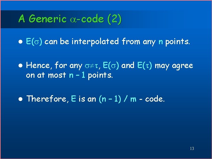
A Generic -code (2) l E( ) can be interpolated from any n points. l Hence, for any , E( ) and E( ) may agree on at most n – 1 points. l Therefore, E is an (n – 1) / m - code. 13

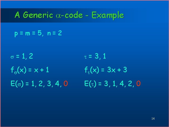
A Generic -code - Example p = m = 5, n = 2 = 1, 2 = 3, 1 f (x) = x + 1 f (x) = 3 x + 3 E( ) = 1, 2, 3, 4, 0 E( ) = 3, 1, 4, 2, 0 14

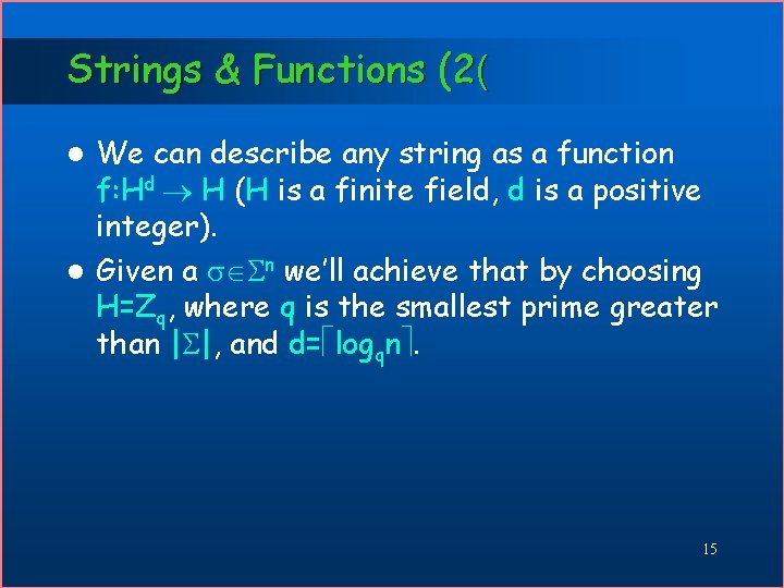
Strings & Functions (2( We can describe any string as a function f: Hd H (H is a finite field, d is a positive integer). l Given a n we’ll achieve that by choosing H=Zq, where q is the smallest prime greater than | |, and d= logqn. l 15

Multivariate Polynomials Definition (polynomial): Let F be a field and let d be some positive integer number. A function p: Fd F is a polynomial if it can be written as for some series of coefficients in the field. h is the degree-bound on each one of the variables. The total-degree of the polynomial is max{ i 0+…+id-1 : ai …i 0 }. 0 d-1 16

-Codes - Home Assignment We’ve seen that univariate polynomials over a finite field F with degree-bound r are -codes for = (r-1)/|F|. l For which multivariate polynomials (over a finite field F, with degree-bound h in each variable and dimension d) are -codes? l Next 17

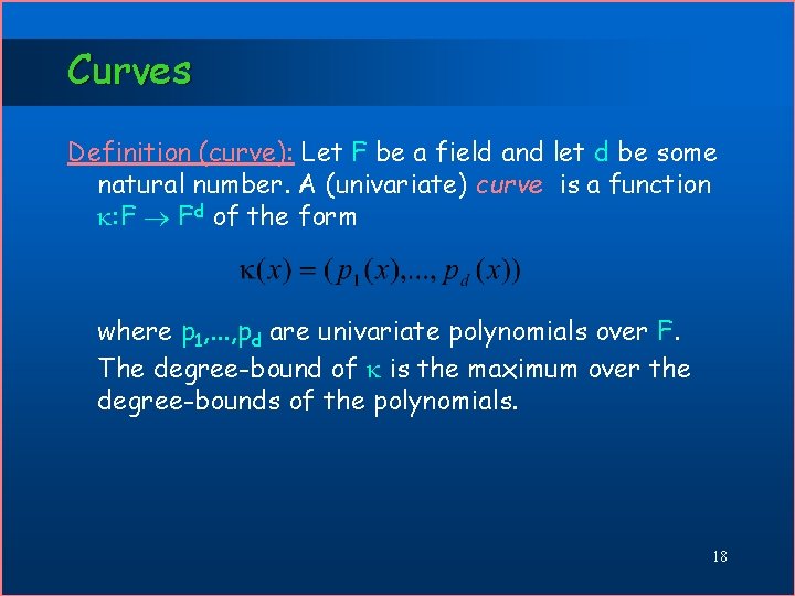
Curves Definition (curve): Let F be a field and let d be some natural number. A (univariate) curve is a function : F Fd of the form where p 1, . . . , pd are univariate polynomials over F. The degree-bound of is the maximum over the degree-bounds of the polynomials. 18

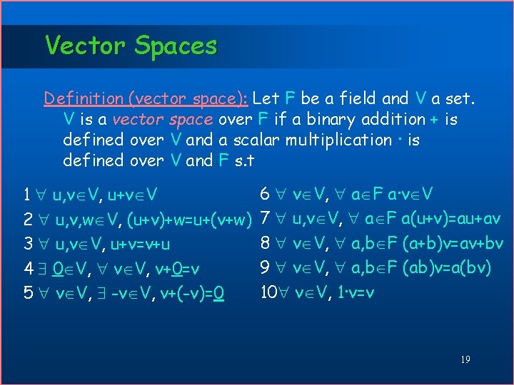
Vector Spaces Definition (vector space): Let F be a field and V a set. V is a vector space over F if a binary addition + is defined over V and a scalar multiplication · is defined over V and F s. t 1 u, v V, u+v V 2 u, v, w V, (u+v)+w=u+(v+w) 3 u, v V, u+v=v+u 4 0 V, v V, v+0=v 5 v V, -v V, v+(-v)=0 6 v V, a F a·v V 7 u, v V, a F a(u+v)=au+av 8 v V, a, b F (a+b)v=av+bv 9 v V, a, b F (ab)v=a(bv) 10 v V, 1·v=v 19

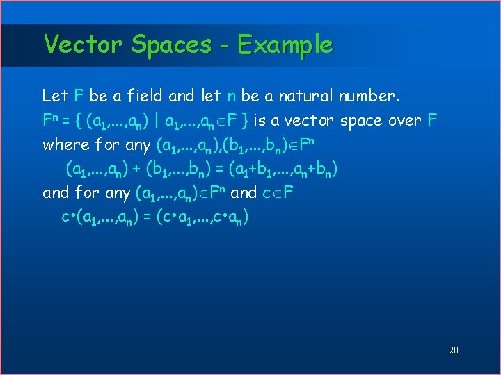
Vector Spaces - Example Let F be a field and let n be a natural number. Fn = { (a 1, . . . , an) | a 1, . . . , an F } is a vector space over F where for any (a 1, . . . , an), (b 1, . . . , bn) Fn (a 1, . . . , an) + (b 1, . . . , bn) = (a 1+b 1, . . . , an+bn) and for any (a 1, . . . , an) Fn and c F c • (a 1, . . . , an) = (c • a 1, . . . , c • an) 20

Subspaces Definition (subspace): A subset W of a vector space V (over a field F) is called a subspace of V if W itself is a vector space over the addition and scalar multiplication operations of V. 21

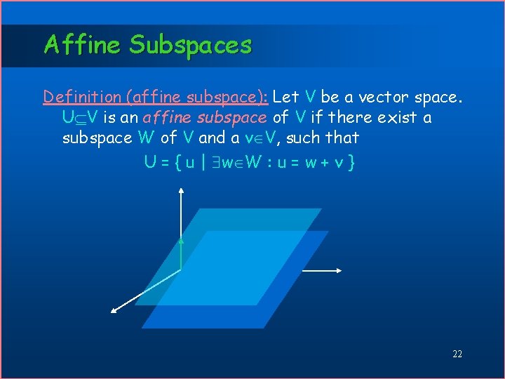
Affine Subspaces Definition (affine subspace): Let V be a vector space. U V is an affine subspace of V if there exist a subspace W of V and a v V, such that U = { u | w W : u = w + v } 22

Linear Combinations Definition (linear combination): Let V be a vector space over some field F. Let v 1, . . . , vk V and let a 1, . . . , ak F. The sum a 1 v 1+. . . +akvk is called a linear combination of v 1, . . . , vk with the coefficients a 1, . . . , ak. Definition (linear dependent): A set of vectors {v 1, . . . , vk} in some vector space V over a field F is linear dependent if there exist a 1, . . . , ak F and an 1 i k for which ai 0, s. t a 1 v 1+. . . +akvk=0. Vectors which are not linear dependent are called linear independent. 23

Basis Definition (Span): Let V be a vector space over some field F. Let K V. Span(K) denotes the subspace of all the linear combination of members of K. Definition (Basis): Let B {0} be a subset of a vector space V. B is called a basis for V if (a) B is linear independent. (b) Span(B)=V. 24

Dimensions Definition (dimension): The number of vectors in any basis of a vector space is called its dimension. Similarly, the dimension of an affine subspace is the dimension of its corresponding subspace. 25

Restriction of Polynomials Definition (restriction of a polynomial to an affine subspace): Let U be an affine subspace of Fd (where F is a field and d is a positive integer). Let p: Fd F be a polynomial. The restriction of p to U is p’: U F, u U p’(u)=p(u). Definition (restriction of a polynomial to a curve): Let : F Fd be a curve (where F is a field and d is a positive integer). Let p: Fd F be a polynomial. The restriction of p to is p’(x)=p( (x)). 26

Restriction of Polynomials Home Assignment [1] Prove that the restriction of p to U is a polynomial. What are its degree-bound and dimension? [2] The same for . Next 27

Low Degree Extension (LDE( Definition (low degree extension): Let : Hd H be a string (where H is some finite field). Given a finite field F, which is a superset of H, we define a low degree extension of to F as a polynomial LDE : Fd F which satisfies: · LDE agrees with on Hd (extension). · The degree-bound of LDE is |H| in each variable (low degree). 28

LDE - Home Assignment Let {0, 1}n. Write down an expression for LDE. 29

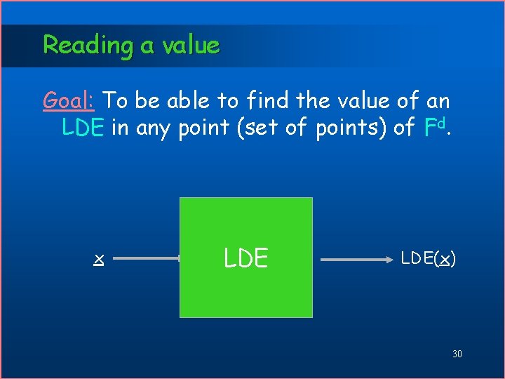
Reading a value Goal: To be able to find the value of an LDE in any point (set of points) of Fd. x LDE(x) 30

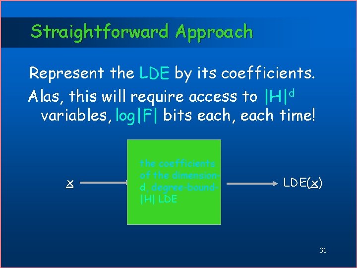
Straightforward Approach Represent the LDE by its coefficients. Alas, this will require access to |H|d variables, log|F| bits each, each time! x the coefficients of the dimensiond, degree-bound|H| LDE(x) 31

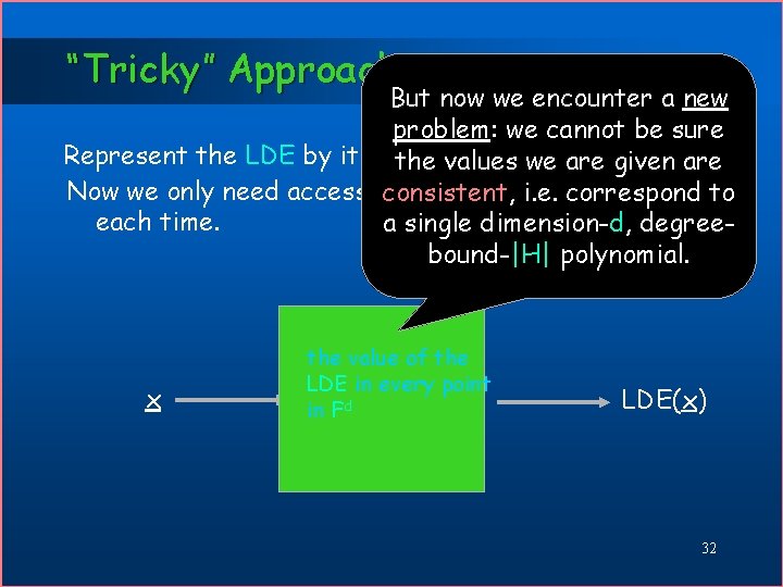
“Tricky” Approach But now we encounter a new problem: we cannot be sure Represent the LDE by its values in thewe points of Fd. are the values are given Now we only need access to one variable bits)to consistent, i. e. (log|F| correspond each time. a single dimension-d, degreebound-|H| polynomial. x the value of the LDE in every point in Fd LDE(x) 32

Consistent Readers In the upcoming lectures we’ll see how to build readers which: l access only a small number of the variables each time. l detect inconsistency with high probability. We’ll later weaken this notion 33

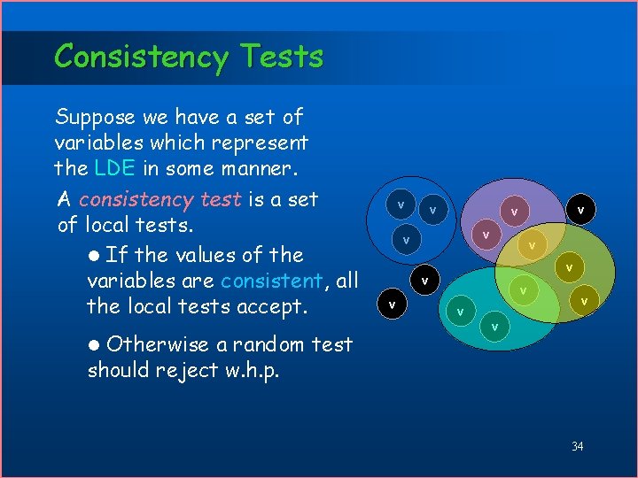
Consistency Tests Suppose we have a set of variables which represent the LDE in some manner. A consistency test is a set of local tests. l If the values of the variables are consistent, all the local tests accept. Otherwise a random test should reject w. h. p. v v v v l 34

Corresponding Game Prover sets values to all variables in the representation. l Verifier picks randomly a single local-test and accepts or rejects according to its output. l The error-probability of a test is the fraction of local tests that may accept although the assigned values do not conform to global consistency. l 35

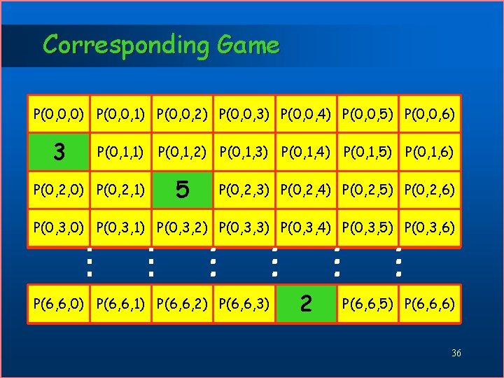
Corresponding Game P(0, 0, 0) P(0, 0, 1) P(0, 0, 2) P(0, 0, 3) P(0, 0, 4) P(0, 0, 5) P(0, 0, 6) 3 P(0, 1, 0) P(0, 1, 1) P(0, 1, 2) P(0, 1, 3) P(0, 1, 4) P(0, 1, 5) P(0, 1, 6) 5 P(0, 2, 0) P(0, 2, 1) P(0, 2, 2) P(0, 2, 3) P(0, 2, 4) P(0, 2, 5) P(0, 2, 6) P(0, 3, 0) P(0, 3, 1) P(0, 3, 2) P(0, 3, 3) P(0, 3, 4) P(0, 3, 5) P(0, 3, 6) 2 P(6, 6, 0) P(6, 6, 1) P(6, 6, 2) P(6, 6, 3) P(6, 6, 4) P(6, 6, 5) P(6, 6, 6) 36