1 Outline Introduction Background Relational database systems Computer
1 Outline Introduction Background Relational database systems Computer networks Distributed Database Design Database Integration Semantic Data Control Distributed Query Processing Multidatabase Query Processing Distributed Transaction Management Data Replication Parallel Database Systems Distributed Object DBMS Peer-to-Peer Data Management Web Data Management Current Issues
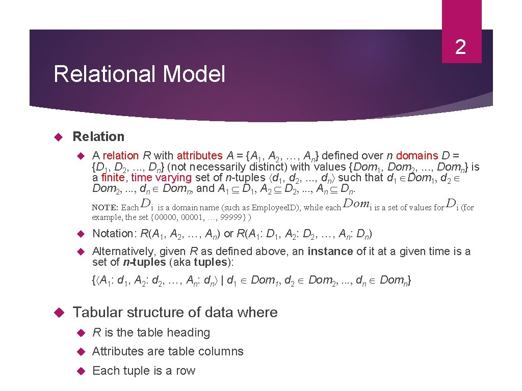
2 Relational Model Relation A relation R with attributes A = {A 1, A 2, …, An} defined over n domains D = {D 1, D 2, . . . , Dn} (not necessarily distinct) with values {Dom 1, Dom 2, . . . , Domn} is a finite, time varying set of n-tuples d 1, d 2, . . . , dn such that d 1 Dom 1, d 2 Dom 2, . . . , dn Domn, and A 1 D 1, A 2 D 2, . . . , An Dn. NOTE: Each Di is a domain name (such as Employee. ID), while each Domi is a set of values for Di (for example, the set {00000, 00001, …, 99999} ) Notation: R(A 1, A 2, …, An) or R(A 1: D 1, A 2: D 2, …, An: Dn) Alternatively, given R as defined above, an instance of it at a given time is a set of n-tuples (aka tuples): { A 1: d 1, A 2: d 2, …, An: dn | d 1 Dom 1, d 2 Dom 2, . . . , dn Domn} Tabular structure of data where R is the table heading Attributes are table columns Each tuple is a row
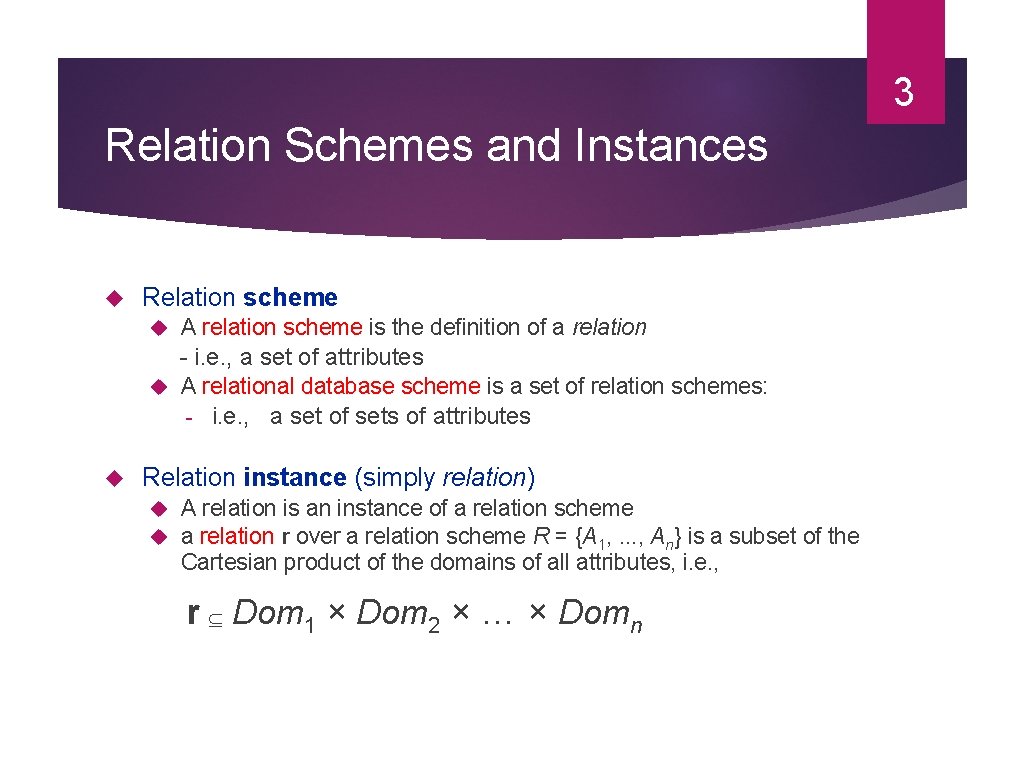
3 Relation Schemes and Instances Relation scheme A relation scheme is the definition of a relation - i. e. , a set of attributes A relational database scheme is a set of relation schemes: - i. e. , a set of sets of attributes Relation instance (simply relation) A relation is an instance of a relation scheme a relation r over a relation scheme R = {A 1, . . . , An} is a subset of the Cartesian product of the domains of all attributes, i. e. , r Dom 1 × Dom 2 × … × Domn

4 Domains A domain is a type in the programming language sense Name: String Salary: Real Domain values is a set of acceptable values for a variable of a given type. Name: Cdn. Names = {…}, Salary: Prof. Salary = {45, 000 - 150, 000} Simple/Composite domains Address = Street name + street number + city + province + postal code Domain compatibility Binary operations (e. g. , comparison to one another, addition, etc. ) can be performed on compatible domains.
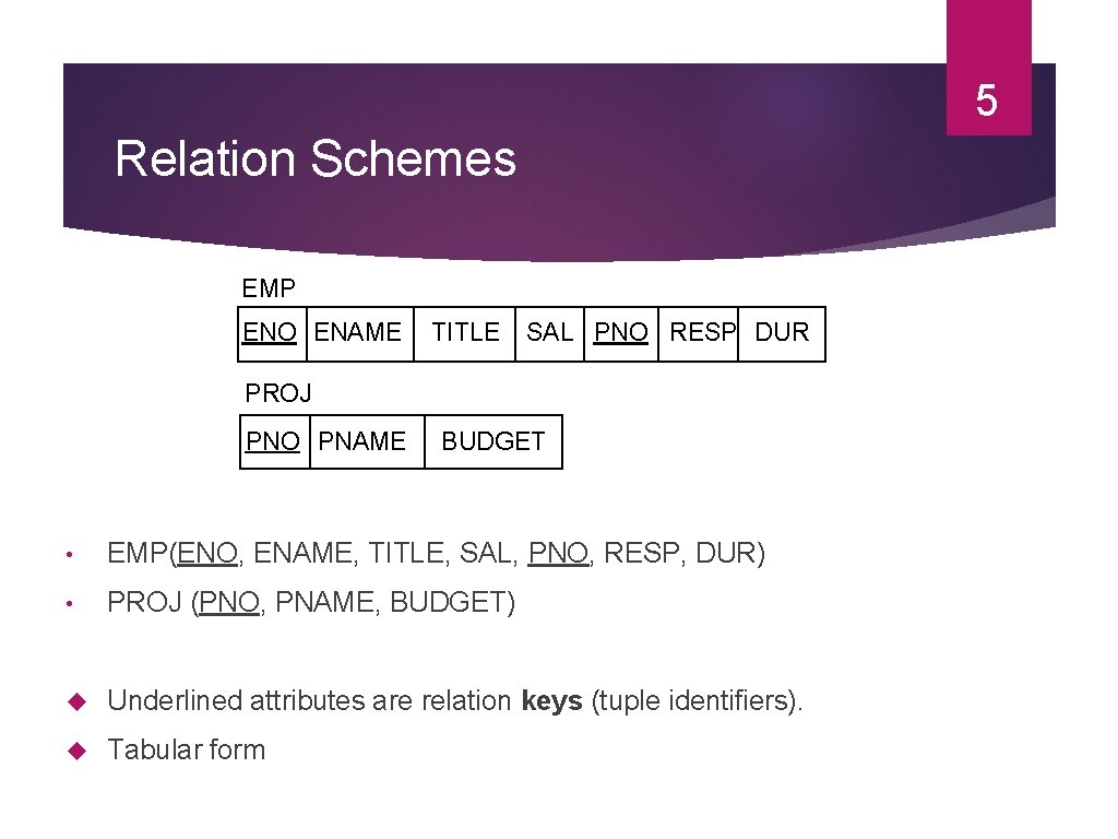
5 Relation Schemes EMP ENO ENAME TITLE SAL PNO RESP DUR PROJ PNO PNAME BUDGET • EMP(ENO, ENAME, TITLE, SAL, PNO, RESP, DUR) • PROJ (PNO, PNAME, BUDGET) Underlined attributes are relation keys (tuple identifiers). Tabular form
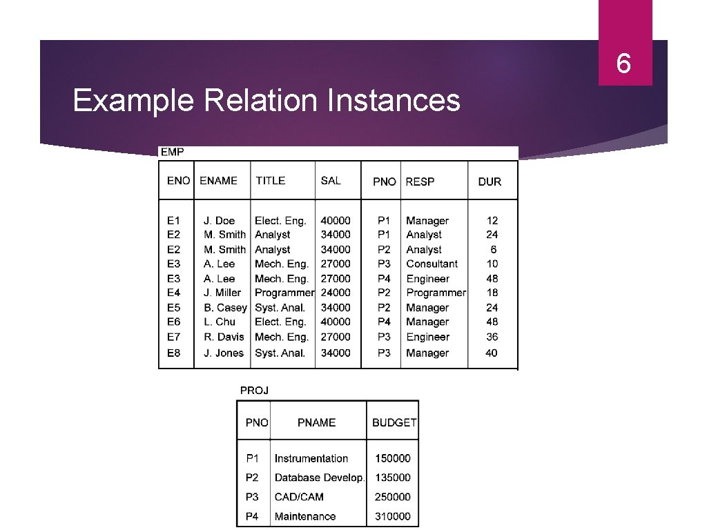
6 Example Relation Instances
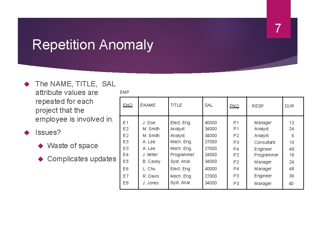
7 Repetition Anomaly The NAME, TITLE, SAL EMP attribute values are repeated for each ENO project that the employee is involved in. E 1 Issues? Waste of space Complicates updates ENAME TITLE SAL E 2 J. Doe M. Smith Elect. Eng. Analyst 40000 34000 P 1 Manager Analyst E 2 E 3 M. Smith A. Lee Analyst Mech. Eng. 34000 27000 P 2 Analyst P 3 Consultant 10 E 3 E 4 A. Lee J. Miller Mech. Eng. Programmer 27000 24000 P 4 P 2 Engineer Programmer 48 18 E 5 B. Casey Syst. Anal. 34000 P 2 Manager 24 E 6 L. Chu Elect. Eng. 40000 P 4 Manager 48 E 7 R. Davis 27000 P 3 Engineer 36 E 8 J. Jones Mech. Eng. Syst. Anal. 34000 P 3 Manager 40 PNO RESP DUR 12 24 6
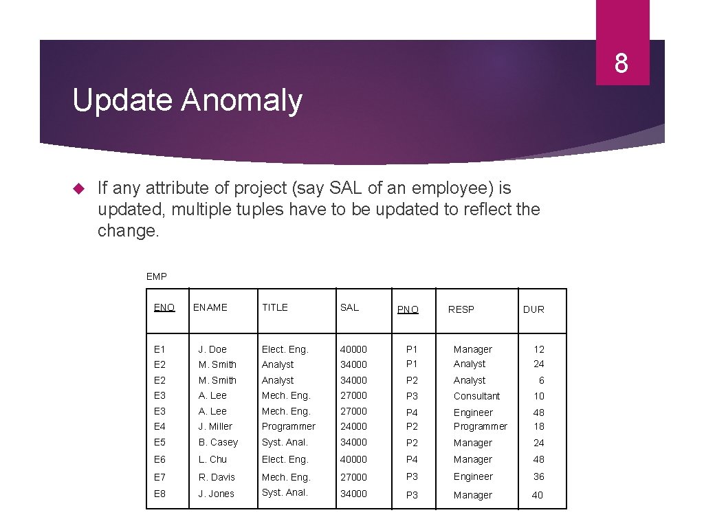
8 Update Anomaly If any attribute of project (say SAL of an employee) is updated, multiple tuples have to be updated to reflect the change. EMP ENO ENAME TITLE SAL PNO RESP DUR E 1 J. Doe Elect. Eng. 40000 P 1 Manager 12 E 2 M. Smith Analyst 34000 P 1 Analyst 24 E 2 M. Smith Analyst 34000 P 2 Analyst 6 E 3 A. Lee Mech. Eng. 27000 P 3 Consultant 10 E 3 A. Lee Mech. Eng. 27000 E 4 J. Miller Programmer 24000 P 4 P 2 Engineer Programmer 48 18 E 5 B. Casey Syst. Anal. 34000 P 2 Manager 24 E 6 L. Chu Elect. Eng. 40000 P 4 Manager 48 E 7 R. Davis Mech. Eng. 27000 P 3 Engineer 36 E 8 J. Jones Syst. Anal. 34000 P 3 Manager 40
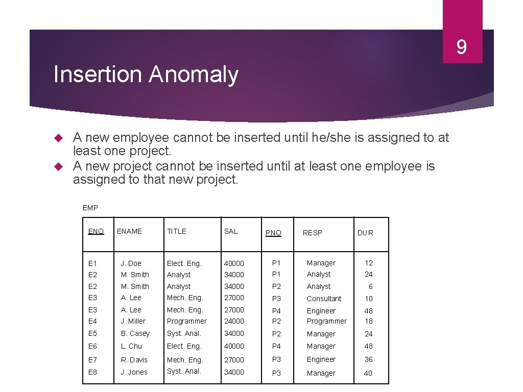
9 Insertion Anomaly A new employee cannot be inserted until he/she is assigned to at least one project. A new project cannot be inserted until at least one employee is assigned to that new project. EMP ENO ENAME TITLE SAL PNO RESP DUR E 1 J. Doe Elect. Eng. 40000 P 1 Manager 12 E 2 M. Smith Analyst 34000 P 1 Analyst 24 E 2 M. Smith Analyst 34000 P 2 Analyst 6 E 3 A. Lee Mech. Eng. 27000 P 3 Consultant 10 E 3 A. Lee Mech. Eng. 27000 E 4 J. Miller Programmer 24000 P 4 P 2 Engineer Programmer 48 18 E 5 B. Casey Syst. Anal. 34000 P 2 Manager 24 E 6 L. Chu Elect. Eng. 40000 P 4 Manager 48 E 7 R. Davis Mech. Eng. 27000 P 3 Engineer 36 E 8 J. Jones Syst. Anal. 34000 P 3 Manager 40
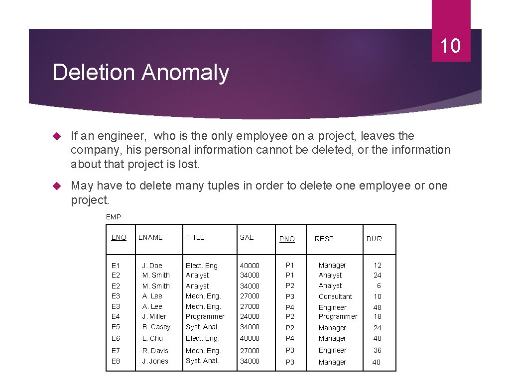
10 Deletion Anomaly If an engineer, who is the only employee on a project, leaves the company, his personal information cannot be deleted, or the information about that project is lost. May have to delete many tuples in order to delete one employee or one project. EMP ENO ENAME TITLE SAL PNO RESP DUR E 1 E 2 J. Doe M. Smith Elect. Eng. Analyst 40000 34000 P 1 Manager Analyst 12 24 E 2 E 3 M. Smith A. Lee Analyst Mech. Eng. 34000 27000 P 2 Analyst P 3 Consultant 10 E 3 E 4 A. Lee J. Miller Mech. Eng. Programmer 27000 24000 P 4 P 2 Engineer Programmer 48 18 E 5 B. Casey Syst. Anal. 34000 P 2 Manager 24 E 6 L. Chu Elect. Eng. 40000 P 4 Manager 48 E 7 R. Davis 27000 P 3 Engineer 36 E 8 J. Jones Mech. Eng. Syst. Anal. 34000 P 3 Manager 40 6
11 What to do? Take each relation individually and “improve” it in terms of the desired characteristics. Normal forms A relation is in a certain normal form when it satisfies the condition associated with that normal form. Atomic values (1 NF), i. e. , no sets as values Can be defined according to keys and dependencies. Functional Dependencies ( 2 NF, 3 NF, BCNF) Multi-valued dependencies (4 NF) Normalization a process of concept separation which applies a top-down methodology for producing a schema by subsequent refinements and decompositions. Do not combine unrelated sets of facts in one table; each relation should contain an independent set of facts. Universal relation assumption 1 NF to 3 NF; 1 NF to BCNF
12 Normalization Issues How do we decompose a schema into a desirable normal form? What criteria should the decomposed schemas follow in order to preserve the semantics of the original schema? Reconstructability: recover the original relation no spurious joins Lossless decomposition: no information loss Dependency preservation: the constraints (i. e. , dependencies) that hold on the original relation should be enforceable by means of the constraints (i. e. , dependencies) defined on the decomposed relations. What happens to queries? Processing time may increase due to joins Denormalization
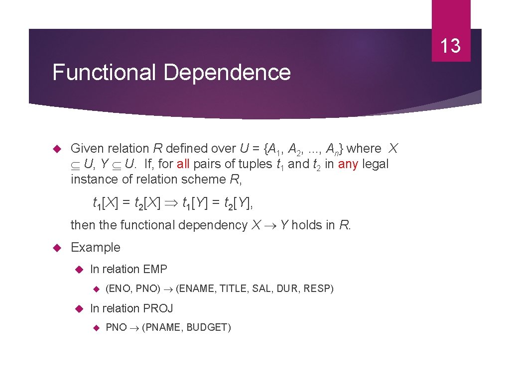
13 Functional Dependence Given relation R defined over U = {A 1, A 2, . . . , An} where X U, Y U. If, for all pairs of tuples t 1 and t 2 in any legal instance of relation scheme R, t 1[X] = t 2[X] t 1[Y] = t 2[Y], then the functional dependency X Y holds in R. Example In relation EMP (ENO, PNO) (ENAME, TITLE, SAL, DUR, RESP) In relation PROJ PNO (PNAME, BUDGET)
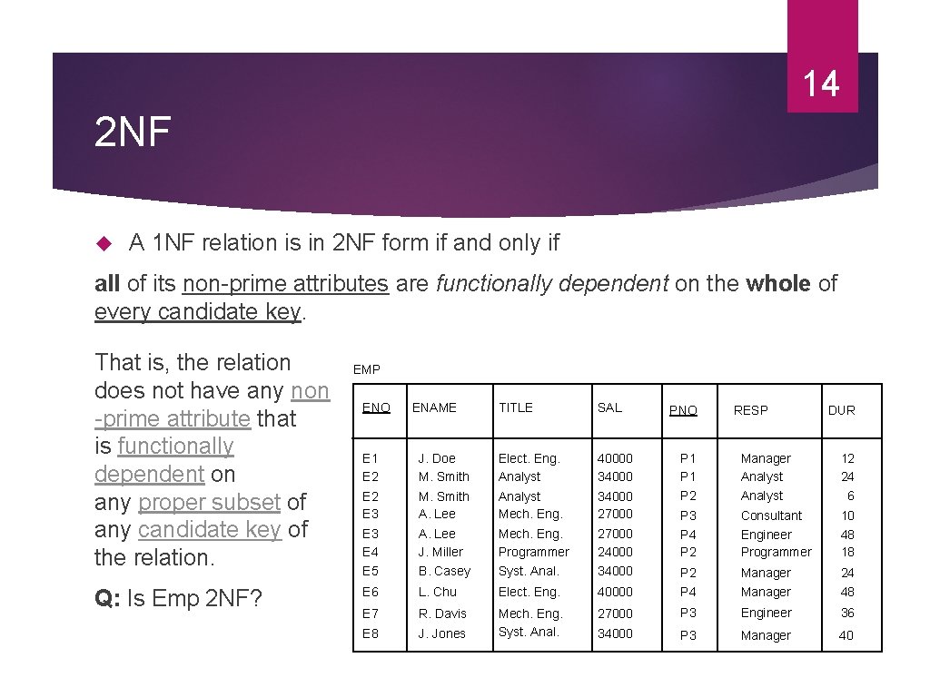
14 2 NF A 1 NF relation is in 2 NF form if and only if all of its non-prime attributes are functionally dependent on the whole of every candidate key. That is, the relation does not have any non -prime attribute that is functionally dependent on any proper subset of any candidate key of the relation. Q: Is Emp 2 NF? EMP ENO ENAME TITLE SAL PNO RESP DUR E 1 E 2 J. Doe M. Smith Elect. Eng. Analyst 40000 34000 P 1 Manager Analyst 12 24 E 2 E 3 M. Smith A. Lee Analyst Mech. Eng. 34000 27000 P 2 Analyst P 3 Consultant 10 E 3 E 4 A. Lee J. Miller Mech. Eng. Programmer 27000 24000 P 4 P 2 Engineer Programmer 48 18 E 5 B. Casey Syst. Anal. 34000 P 2 Manager 24 E 6 L. Chu Elect. Eng. 40000 P 4 Manager 48 E 7 R. Davis 27000 P 3 Engineer 36 E 8 J. Jones Mech. Eng. Syst. Anal. 34000 P 3 Manager 40 6
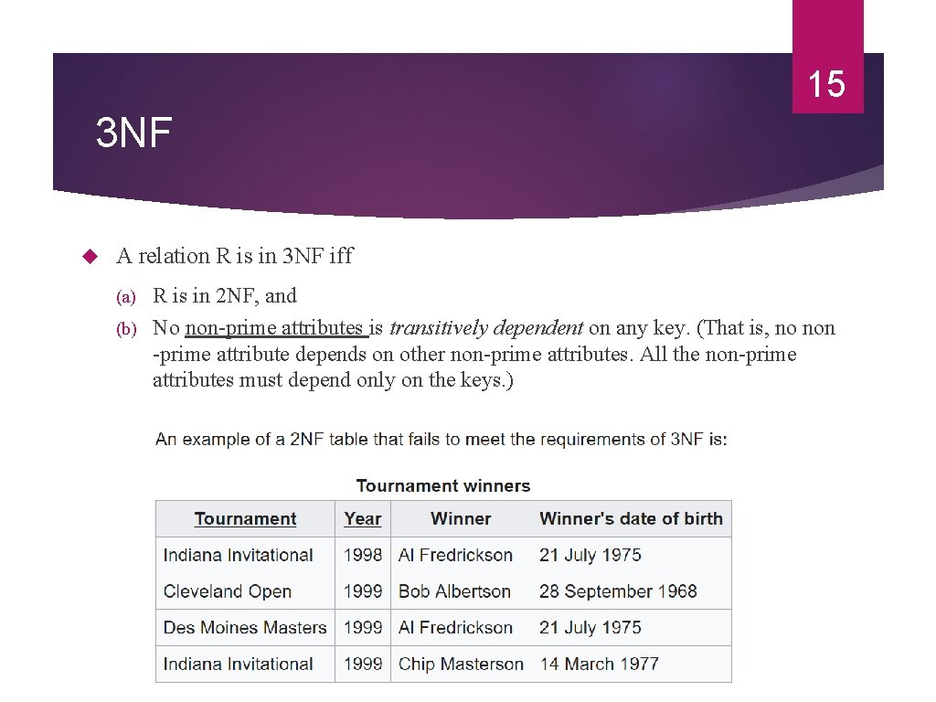
15 3 NF A relation R is in 3 NF iff R is in 2 NF, and (b) No non-prime attributes is transitively dependent on any key. (That is, no non -prime attribute depends on other non-prime attributes. All the non-prime attributes must depend only on the keys. ) (a)
16 BCNF (or 3. 5 NF) A relation R is in BCNF iff (a) R is in 3 NF, and (b) for every one of its dependencies X → Y, at least one of the following conditions hold: X → Y is a trivial functional dependency (Y ⊆ X), X is a superkey for R.
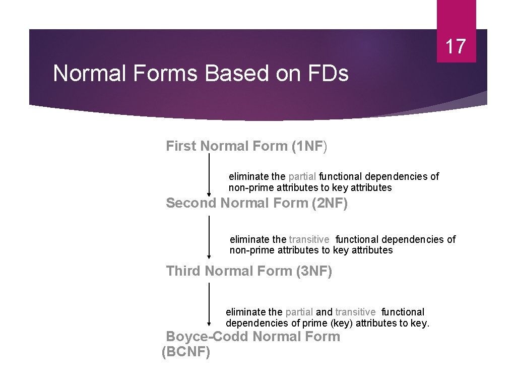
17 Normal Forms Based on FDs First Normal Form (1 NF) eliminate the partial functional dependencies of non-prime attributes to key attributes Second Normal Form (2 NF) eliminate the transitive functional dependencies of non-prime attributes to key attributes Third Normal Form (3 NF) eliminate the partial and transitive functional dependencies of prime (key) attributes to key. Boyce-Codd Normal Form (BCNF)
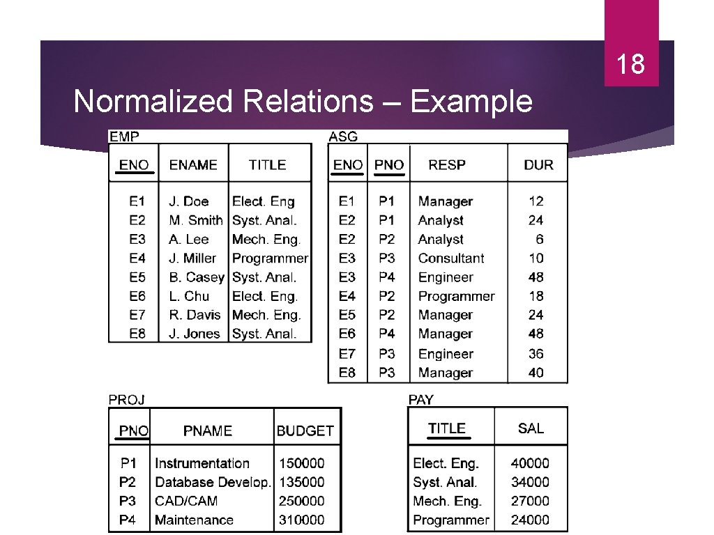
18 Normalized Relations – Example
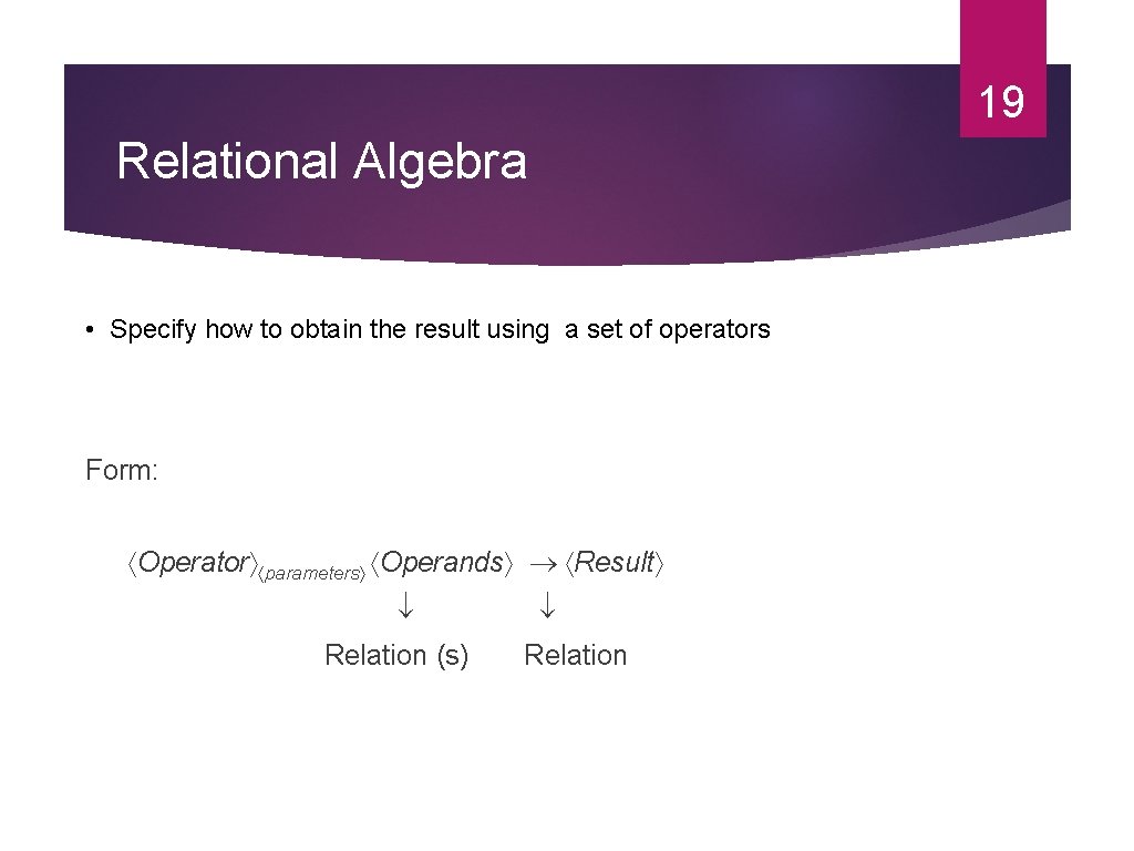
19 Relational Algebra • Specify how to obtain the result using a set of operators Form: Operator parameters Operands Result Relation (s) Relation
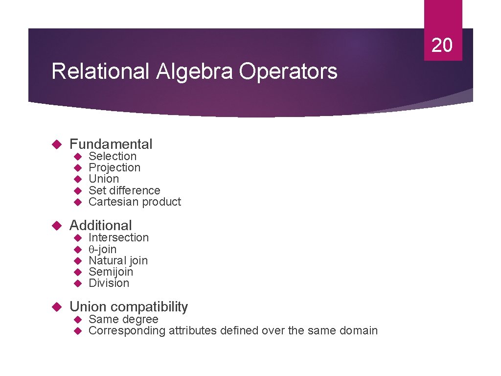
20 Relational Algebra Operators Fundamental Additional Selection Projection Union Set difference Cartesian product Intersection -join Natural join Semijoin Division Union compatibility Same degree Corresponding attributes defined over the same domain
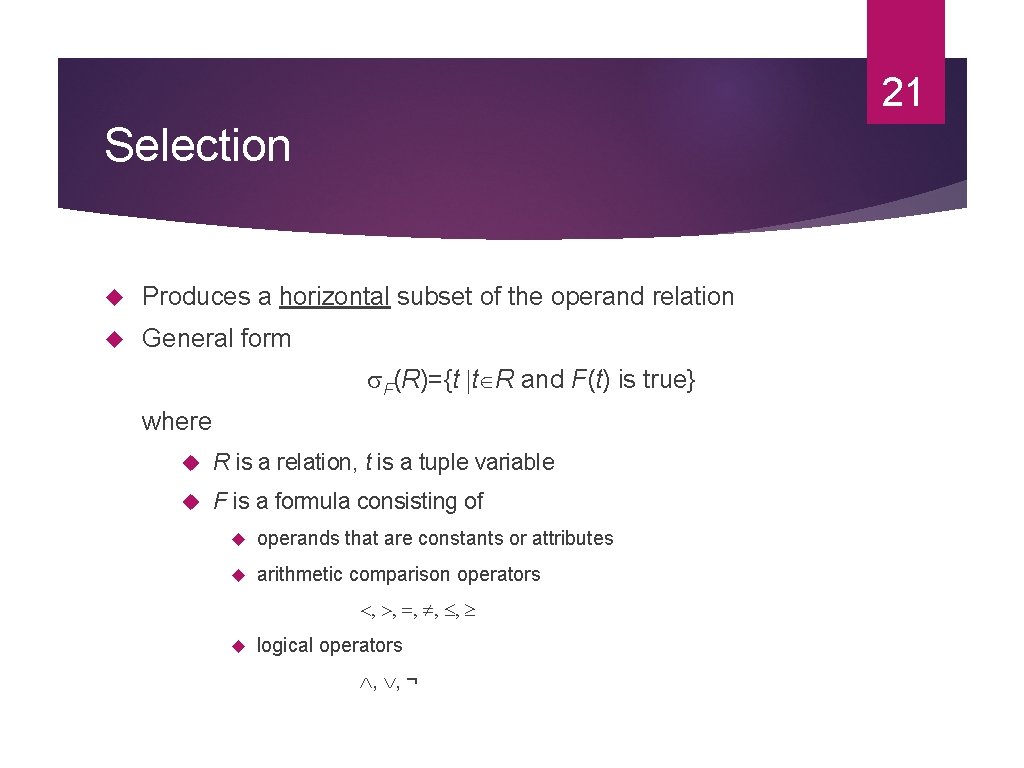
21 Selection Produces a horizontal subset of the operand relation General form F(R)={t t R and F(t) is true} where R is a relation, t is a tuple variable F is a formula consisting of operands that are constants or attributes arithmetic comparison operators <, >, =, , , logical operators , , ¬
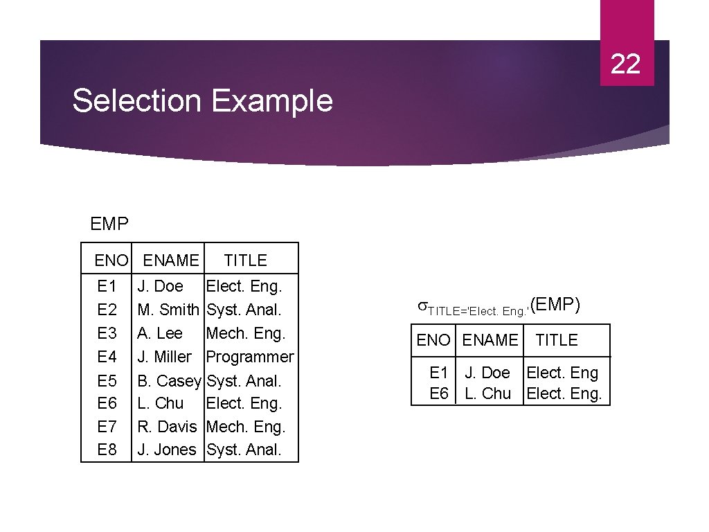
22 Selection Example EMP ENO ENAME E 1 E 2 E 3 E 4 E 5 E 6 E 7 E 8 TITLE J. Doe Elect. Eng. M. Smith Syst. Anal. A. Lee Mech. Eng. J. Miller Programmer B. Casey Syst. Anal. L. Chu Elect. Eng. R. Davis Mech. Eng. J. Jones Syst. Anal. TITLE='Elect. Eng. '(EMP) ENO ENAME TITLE E 1 J. Doe Elect. Eng E 6 L. Chu Elect. Eng.
23 Projection Produces a vertical slice of a relation General form A 1, …, An(R)={t[A 1, …, An] t R} where R is a relation, t is a tuple variable {A 1, …, An} is a subset of the attributes of R over which the projection will be performed Note: projection can generate duplicate tuples. Commercial systems (and SQL) allow this and provide Projection with duplicate elimination Projection without duplicate elimination
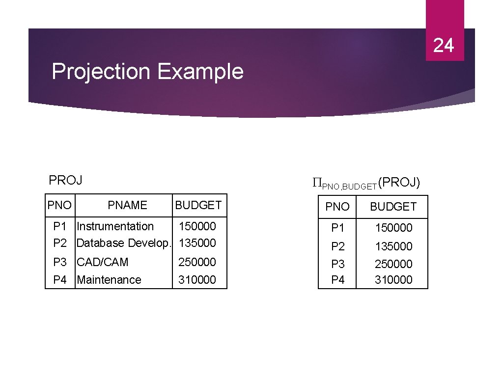
24 Projection Example PROJ PNO, BUDGET(PROJ) PNAME BUDGET PNO BUDGET P 1 Instrumentation 150000 P 2 Database Develop. 135000 P 1 150000 P 2 135000 P 3 CAD/CAM 250000 P 4 Maintenance 310000 P 3 P 4 250000 310000
25 Union Similar to set union General form R S={t t R or t S} where R, S are relations, t is a tuple variable Result contains tuples that are in R or in S, or in both (duplicates removed) R, S should be union-compatible
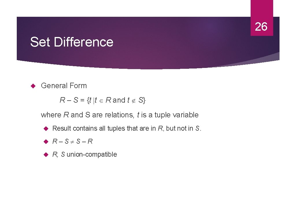
26 Set Difference General Form R – S = {t t R and t S} where R and S are relations, t is a tuple variable Result contains all tuples that are in R, but not in S. R – S S – R R, S union-compatible
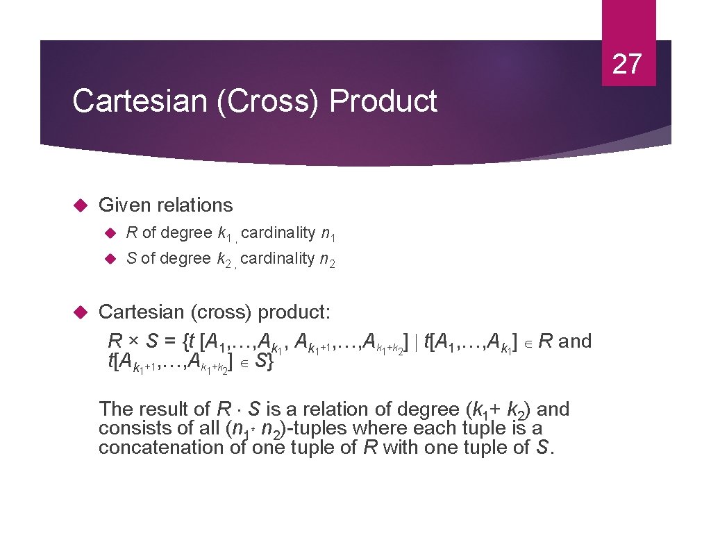
27 Cartesian (Cross) Product Given relations R of degree k 1 , cardinality n 1 S of degree k 2 , cardinality n 2 Cartesian (cross) product: R × S = {t [A 1, …, Ak 1+1, …, Ak 1+k 2] t[A 1, …, Ak 1] R and t[Ak 1+1, …, Ak 1+k 2] S} The result of R × S is a relation of degree (k 1+ k 2) and consists of all (n 1* n 2)-tuples where each tuple is a concatenation of one tuple of R with one tuple of S.
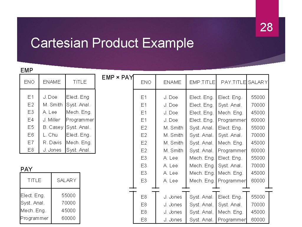
28 Cartesian Product Example EMP ENO ENAME TITLE EMP × PAY ENO ENAME EMP. TITLE PAY. TITLE SALARY E 1 J. Doe Elect. Eng. 55000 E 2 M. Smith Syst. Anal. E 1 J. Doe Elect. Eng. Syst. Anal. 70000 E 3 A. Lee Mech. Eng. E 1 J. Doe Elect. Eng. Mech. Eng. 45000 E 4 J. Miller Programmer E 1 J. Doe Elect. Eng. Programmer 60000 E 5 B. Casey Syst. Anal. E 2 M. Smith Syst. Anal. Elect. Eng. 55000 E 6 L. Chu Elect. Eng. E 2 M. Smith Syst. Anal. 70000 E 7 R. Davis Mech. Eng. E 2 M. Smith Syst. Anal. Mech. Eng. 45000 E 8 J. Jones Syst. Anal. E 2 M. Smith Syst. Anal. Programmer 60000 E 3 A. Lee Mech. Eng. Elect. Eng. 55000 E 3 A. Lee Mech. Eng. Syst. Anal. 70000 E 3 A. Lee Mech. Eng. 45000 SALARY E 3 A. Lee Mech. Eng. Programmer 60000 Elect. Eng. 55000 E 8 J. Jones Syst. Anal. Elect. Eng. 55000 Syst. Anal. 70000 E 8 J. Jones Syst. Anal. 70000 Mech. Eng. 45000 E 8 J. Jones Syst. Anal. Mech. Eng. 45000 Programmer 60000 E 8 J. Jones Syst. Anal. Programmer 60000 PAY TITLE
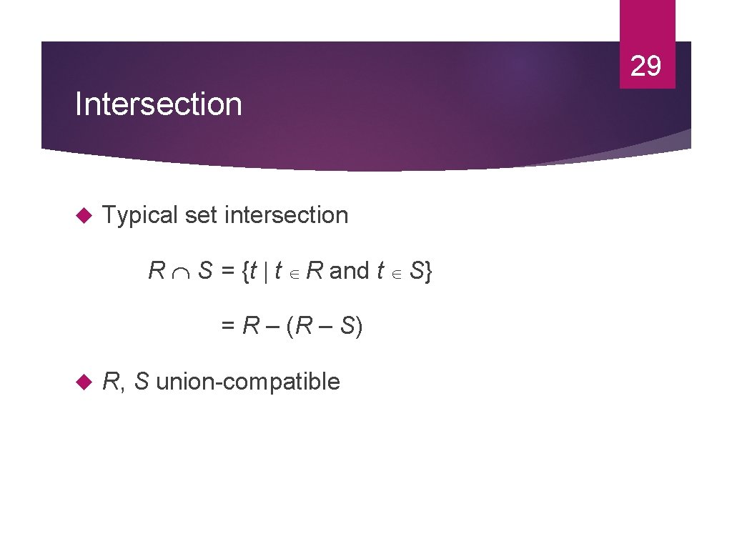
29 Intersection Typical set intersection R S = {t t R and t S} = R – (R – S) R, S union-compatible
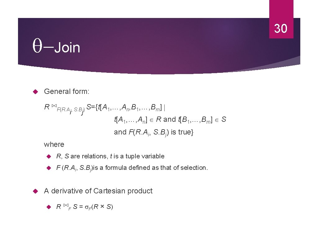
30 -Join General form: R ⋈F(R. A , S. B ) S={t[A 1, …, An, B 1, …, Bm] i j t[A 1, …, An] R and t[B 1, …, Bm] S and F(R. Ai, S. Bj) is true} where R, S are relations, t is a tuple variable F (R. Ai, S. Bj)is a formula defined as that of selection. A derivative of Cartesian product R ⋈F S = F(R × S)
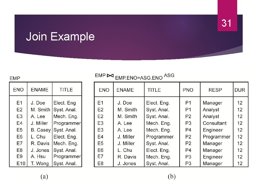
31 Join Example
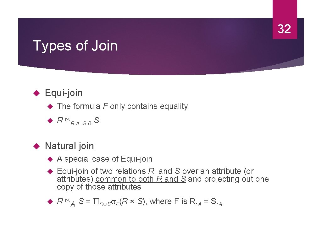
32 Types of Join Equi-join The formula F only contains equality R ⋈R. A=S. B S Natural join A special case of Equi-join of two relations R and S over an attribute (or attributes) common to both R and S and projecting out one copy of those attributes R ⋈A S = R S F(R × S), where F is R. A = S. A
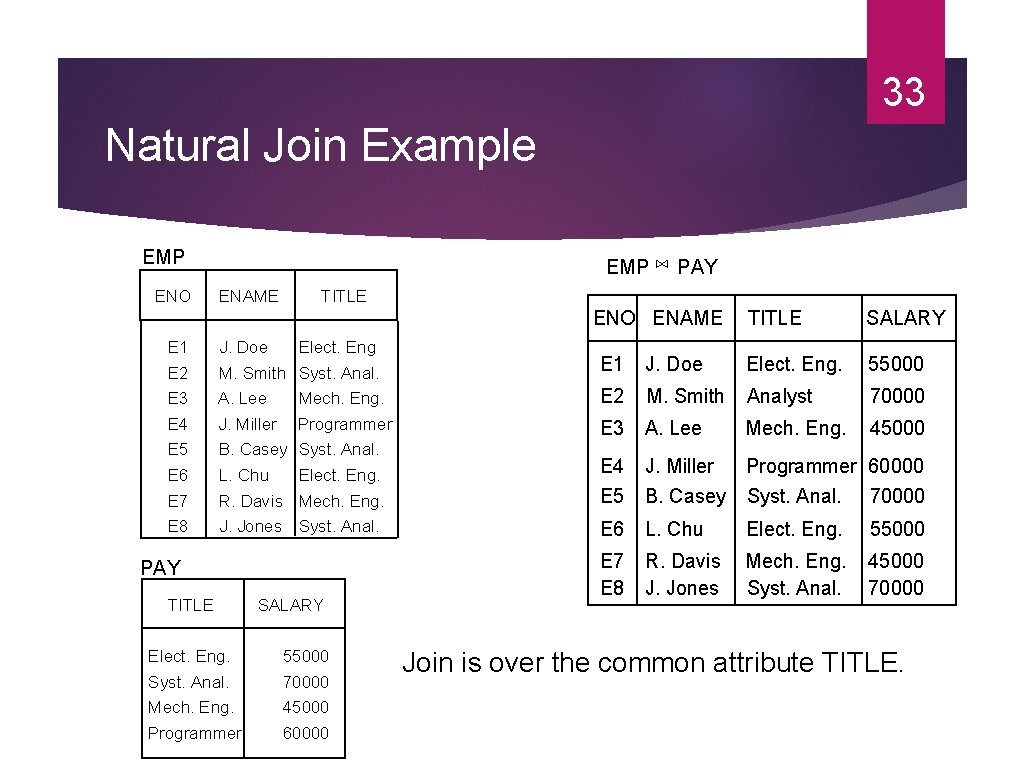
33 Natural Join Example EMP ENO EMP ENAME ⋈ PAY TITLE ENO ENAME Elect. Eng TITLE SALARY E 1 J. Doe E 2 M. Smith Syst. Anal. E 1 J. Doe Elect. Eng. 55000 E 3 A. Lee Mech. Eng. E 2 M. Smith Analyst 70000 E 4 J. Miller Programmer E 3 A. Lee Mech. Eng. 45000 E 5 B. Casey Syst. Anal. E 6 L. Chu Elect. Eng. E 4 J. Miller Programmer 60000 E 7 R. Davis Mech. Eng. E 5 B. Casey Syst. Anal. 70000 E 8 J. Jones Syst. Anal. E 6 L. Chu Elect. Eng. 55000 E 7 E 8 R. Davis J. Jones Mech. Eng. Syst. Anal. 45000 70000 PAY TITLE SALARY Elect. Eng. 55000 Syst. Anal. 70000 Mech. Eng. 45000 Programmer 60000 Join is over the common attribute TITLE.
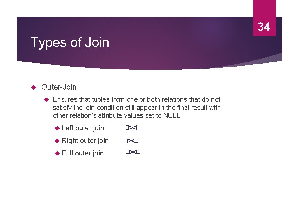
34 Types of Join Outer-Join Ensures that tuples from one or both relations that do not satisfy the join condition still appear in the final result with other relation’s attribute values set to NULL Left outer join Right outer join Full outer join
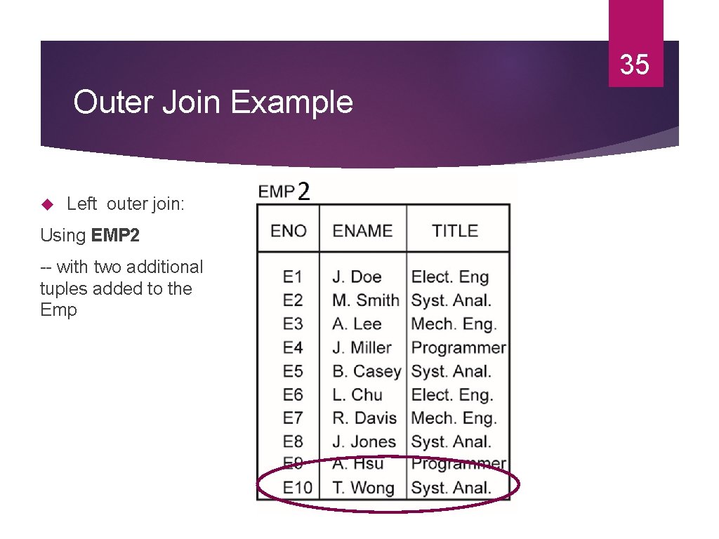
35 Outer Join Example Left outer join: Using EMP 2 -- with two additional tuples added to the Emp
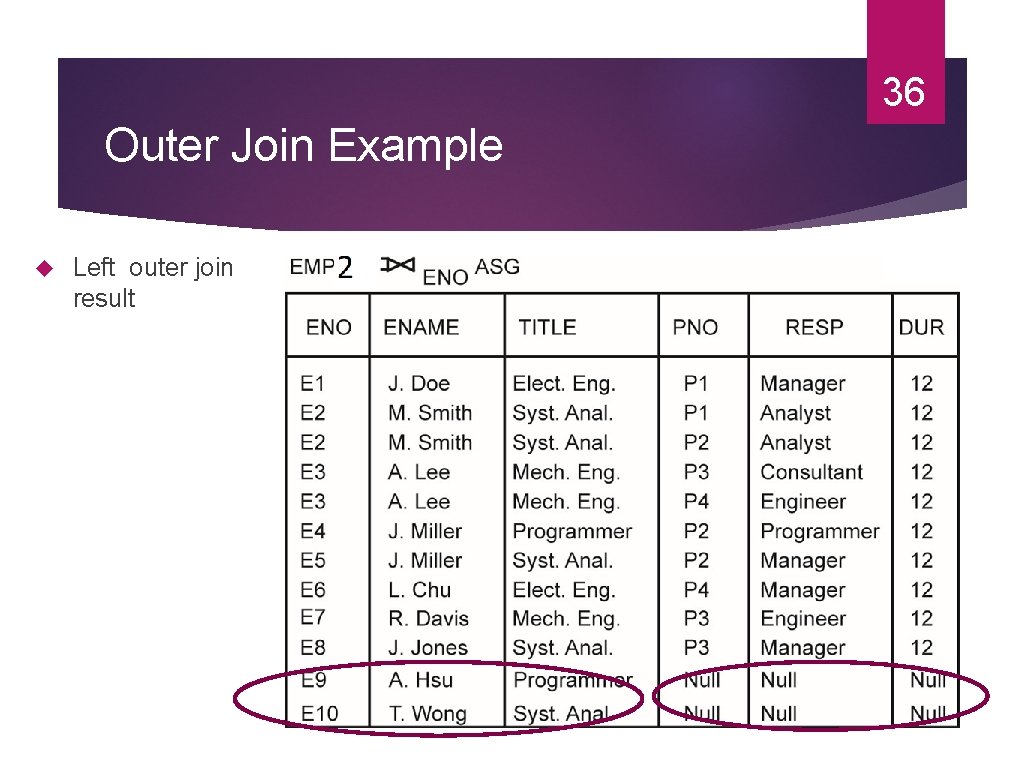
36 Outer Join Example Left outer join result
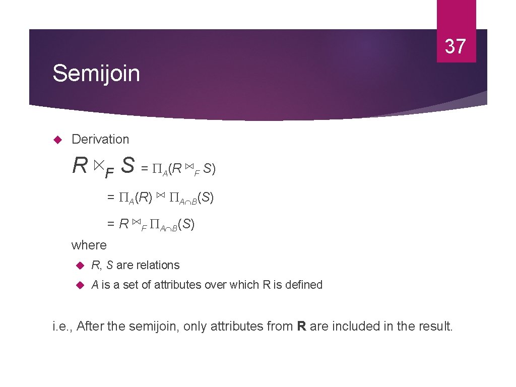
37 Semijoin Derivation R ⋉F S = (R ⋈ A = A(R) = R F S) ⋈ A B(S) ⋈F A B(S) where R, S are relations A is a set of attributes over which R is defined i. e. , After the semijoin, only attributes from R are included in the result.
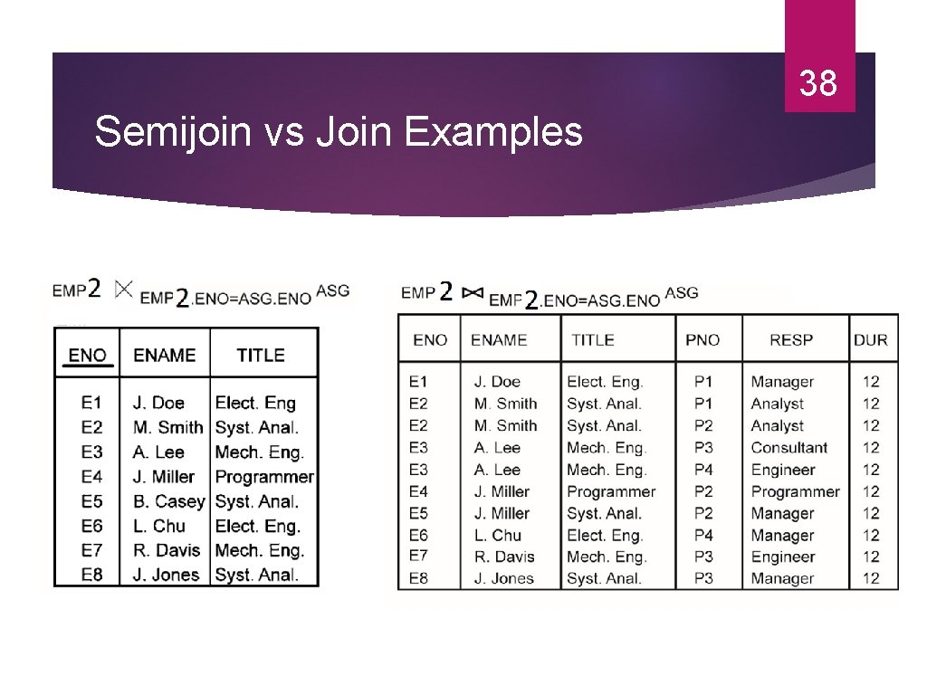
38 Semijoin vs Join Examples
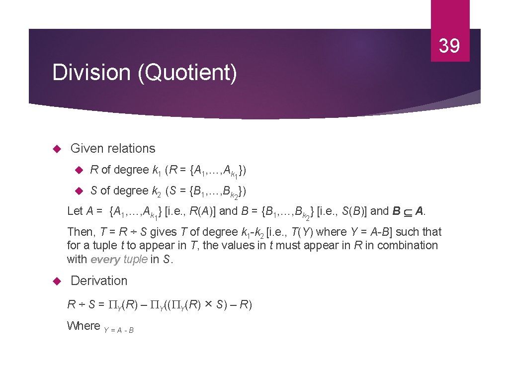
39 Division (Quotient) Given relations R of degree k 1 (R = {A 1, …, Ak 1}) S of degree k 2 (S = {B 1, …, Bk 2}) Let A = {A 1, …, Ak } [i. e. , R(A)] and B = {B 1, …, Bk } [i. e. , S(B)] and B A. 1 2 Then, T = R ÷ S gives T of degree k 1 -k 2 [i. e. , T(Y) where Y = A-B] such that for a tuple t to appear in T, the values in t must appear in R in combination with every tuple in S. Derivation R ÷ S = Y(R) – Y(( Y(R) Where Y = A - B × S) – R)
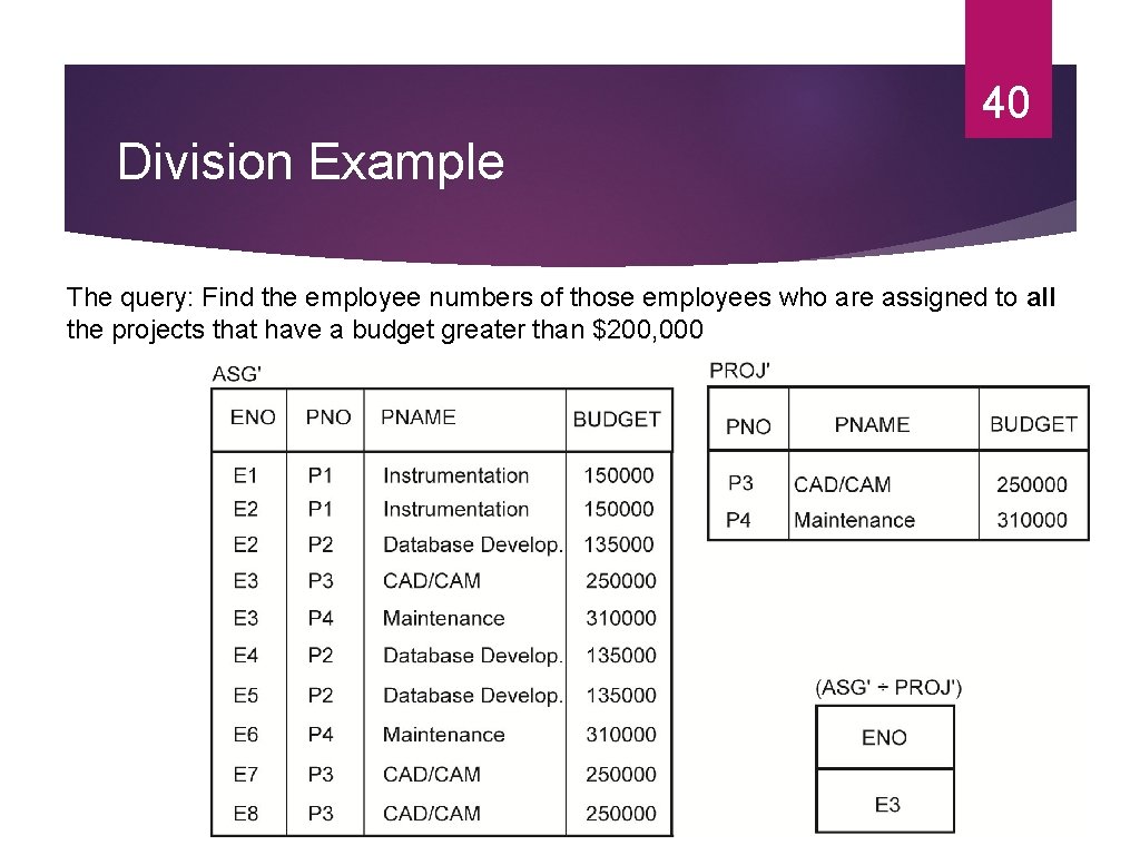
40 Division Example The query: Find the employee numbers of those employees who are assigned to all the projects that have a budget greater than $200, 000
41 Relational Calculus Specify the properties that the result should hold Declarative/what (as in Relational Calculus) vs procedural/how (as in Relational Algebra) Two categories: Tuple relational calculus Domain relational calculus
42 Tuple Relational Calculus Query of the form {t|F{t}} where t is a tuple variable F is a well-formed formula Atomic formula Tuple-variable membership expressions R. t or R(t) : tuple t belongs to relation R Conditions s[A] t[B]; s and t are tuple variables, A and B are components of s and t, respectively, {<, >, =, ≠, ≤, ≥}; e. g. , s[SAL] > t[SAL] s[A] c; s, A, and as defined above, c is a constant; e. g. , s[ENAME] = ‘Smith’ SQL is an example of tuple relational calculus (at least in its simple form)
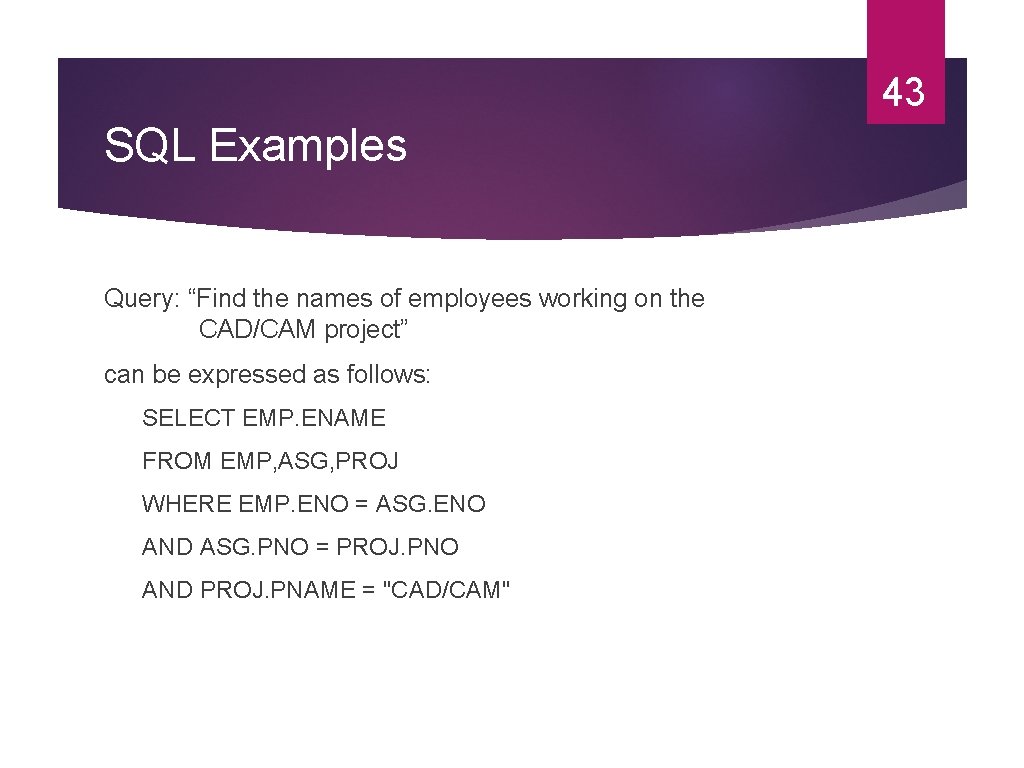
43 SQL Examples Query: “Find the names of employees working on the CAD/CAM project” can be expressed as follows: SELECT EMP. ENAME FROM EMP, ASG, PROJ WHERE EMP. ENO = ASG. ENO AND ASG. PNO = PROJ. PNO AND PROJ. PNAME = "CAD/CAM"
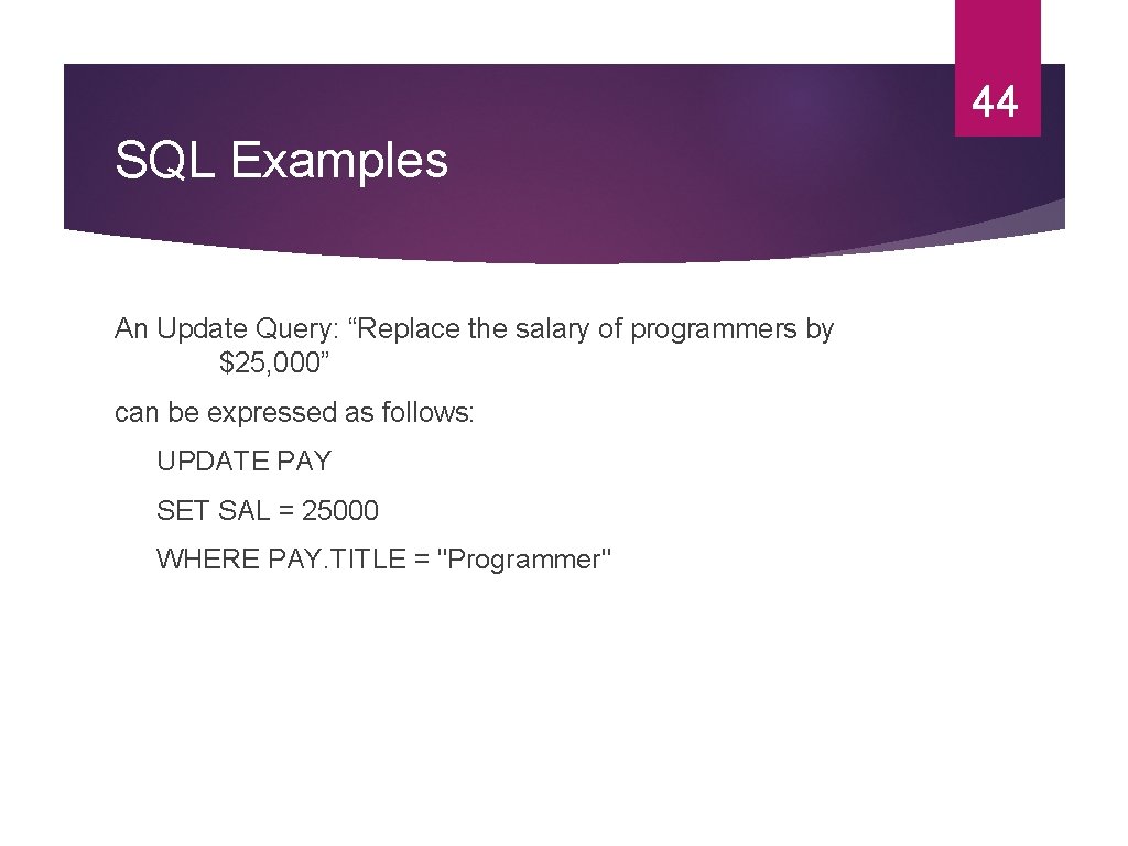
44 SQL Examples An Update Query: “Replace the salary of programmers by $25, 000” can be expressed as follows: UPDATE PAY SET SAL = 25000 WHERE PAY. TITLE = "Programmer"
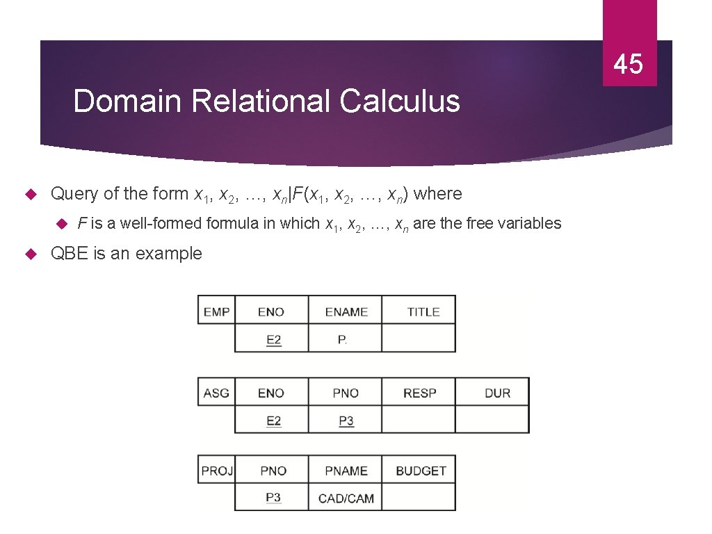
45 Domain Relational Calculus Query of the form x 1, x 2, …, xn|F(x 1, x 2, …, xn) where F is a well-formed formula in which x 1, x 2, …, xn are the free variables QBE is an example
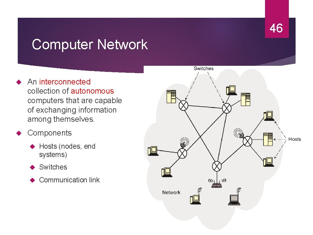
46 Computer Network An interconnected collection of autonomous computers that are capable of exchanging information among themselves. Components Hosts (nodes, end systems) Switches Communication link
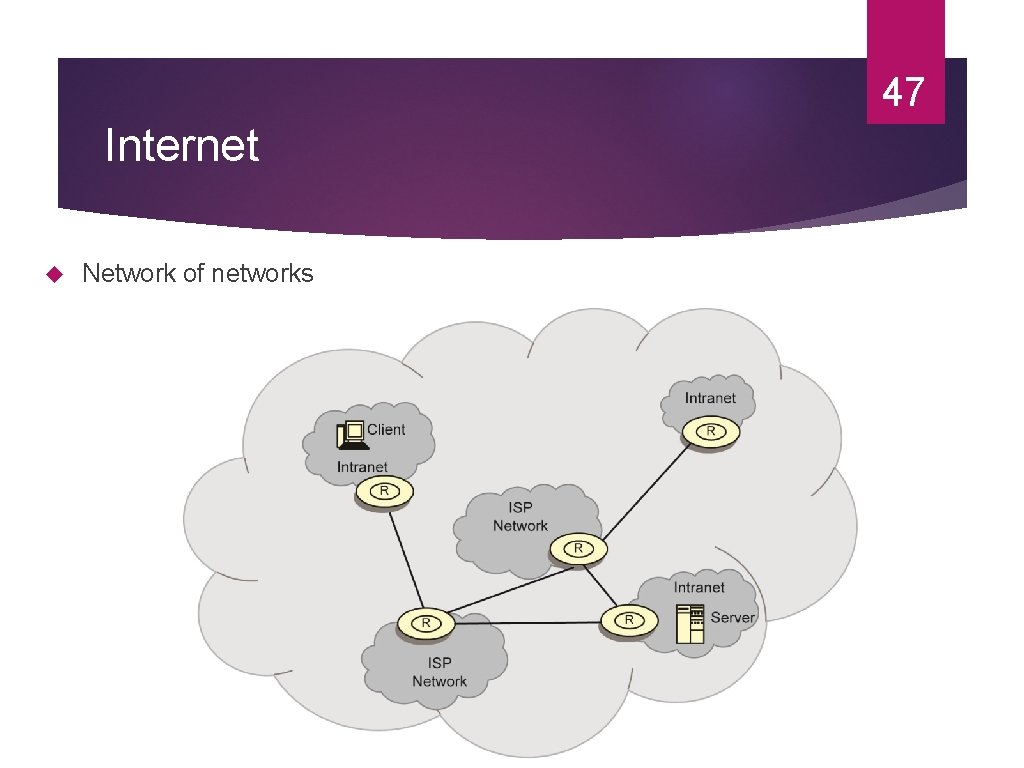
47 Internet Network of networks
48 Types of Networks According to scale (geographic distribution) Wide are network (WAN) Distance between any two nodes > 20 km and can go as high as thousands of kms Long delays due to distance traveled Heterogeneity of transmission media Speeds of 150 Mbps to 10 Gbps (OC 192 on the backbone) Local area network (LAN) Limited in geographic scope (usually < 2 km) Speeds 10 -1000 Mbps Short delays and low noise Metropolitan area network (MAN) In between LAN and WAN
49 Types of Networks (cont’d) Topology Irregular: No regularity in the interconnection – e. g. , Internet Bus: All workstations are connected in succession (a "bus" arrangement) on a single cable. All transmissions go to all the connected workstations. Each workstation then selects the transmissions it should receive based on the address information contained in the transmission. e. g. , 10 BASE 5 (Standard Ethernet) and 10 BASE 2 (Thin Ethernet) Star: All attached workstations are wired directly to a central hub that establishes, maintains, and breaks connections between them (in the event of an error). e. g. , 10 BASE-T (Twisted-Pair Ethernet)
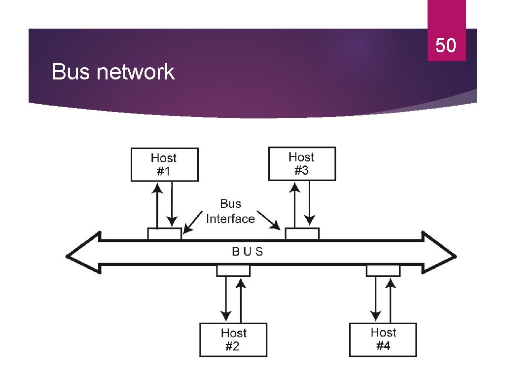
50 Bus network
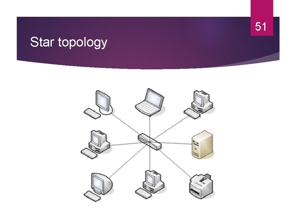
51 Star topology
52 Communication Schemes Point-to-point (unicast) One or more (direct or indirect) links between each pair of nodes Communication always between two nodes Receiver and sender are identified by their addresses included in the message header Message may follow one of many links between the sender and receiver using switching or routing Broadcast (multi-point) Messages are transmitted over a shared channel and received by all the nodes Each node checks the address and if it is not the intended recipient, ignores Multi-cast: special case Message is sent to a subset of the nodes

53 Communication Alternatives Twisted pair Coaxial Fiber optic cable Satellite Microwave Wireless
54 Data Communication Hosts are connected by links, each of which can carry one or more channels Link: physical entity; channel: logical entity Digital signal versus analog signal Capacity – bandwidth The amount of information that can be transmitted over the channel in a given time unit Alternative messaging schemes Packet switching Messages are divided into fixed size packets, each of which is routed from the source to the destination Circuit switching A dedicated channel is established between the sender and receiver for the duration of the session
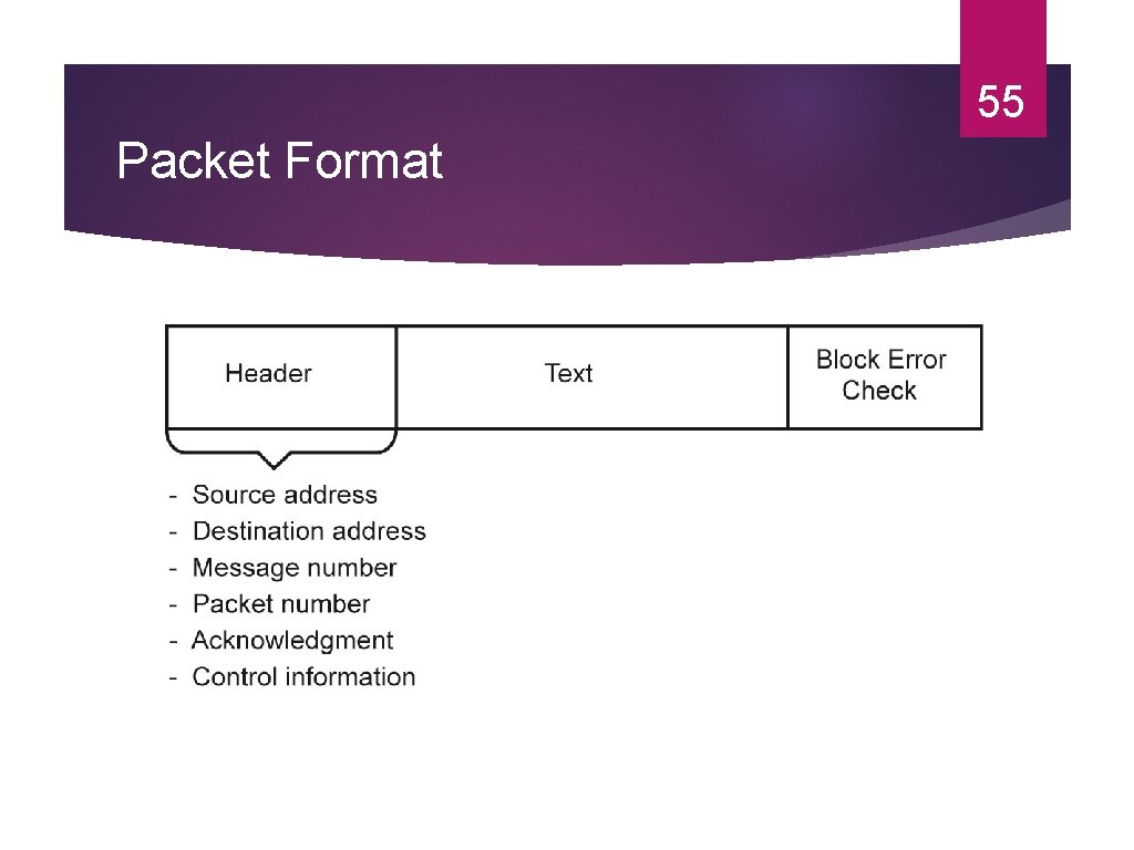
55 Packet Format
56 Communication Protocols Software that ensures error-free, reliable and efficient communication between hosts Layered architecture – hence protocol stack or protocol suite TCP/IP is the best-known one Used in the Internet
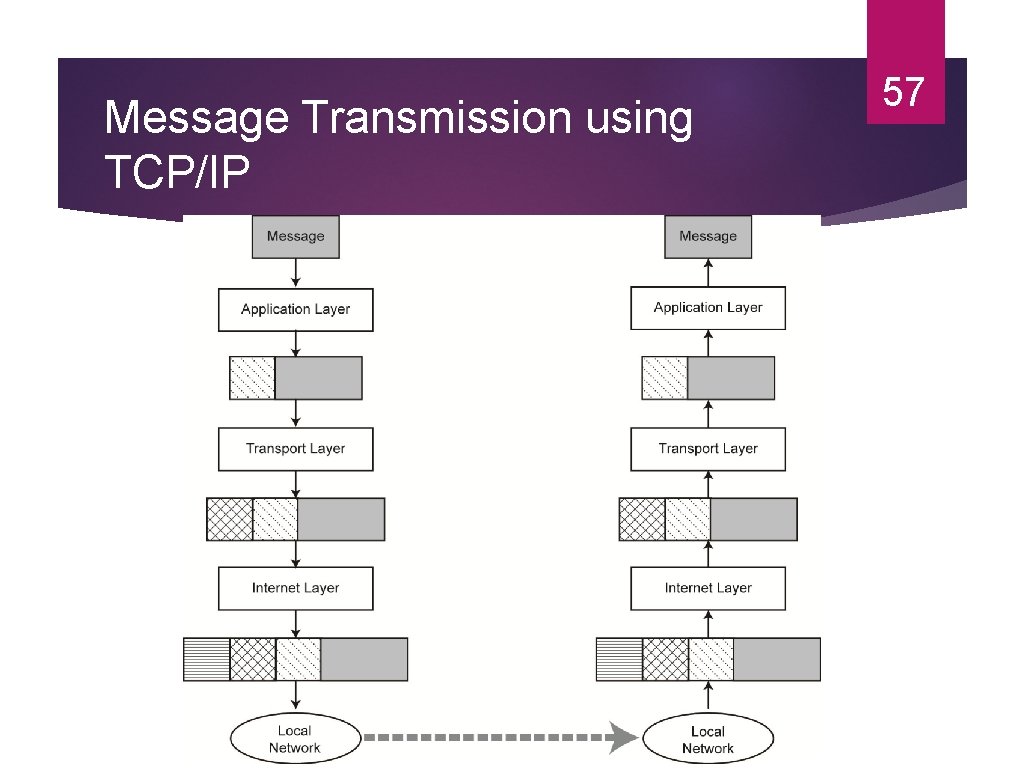
Message Transmission using TCP/IP 57
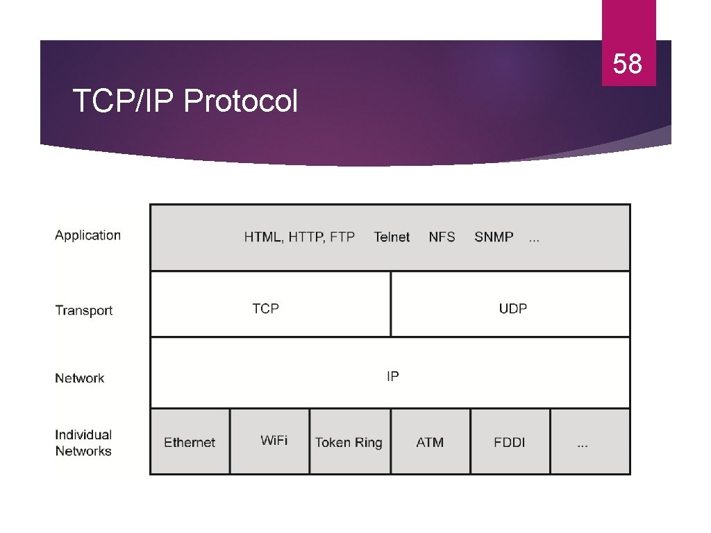
58 TCP/IP Protocol
- Slides: 58