1 Optimizing Stream Programs Using Linear State Space

1 Optimizing Stream Programs Using Linear State Space Analysis Sitij Agrawal 1, 2, William Thies 1, and Saman Amarasinghe 1 1 Massachusetts Institute of Technology 2 Sandbridge Technologies CASES 2005 http: //cag. lcs. mit. edu/streamit

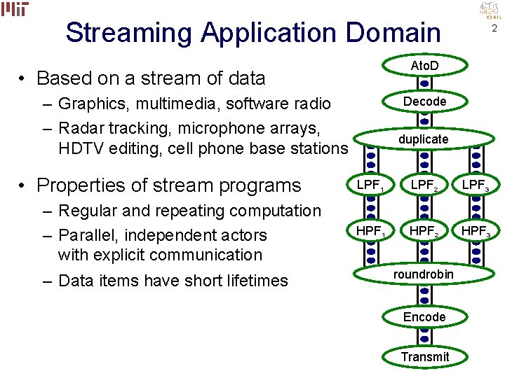
Streaming Application Domain Ato. D • Based on a stream of data – Graphics, multimedia, software radio – Radar tracking, microphone arrays, HDTV editing, cell phone base stations • Properties of stream programs – Regular and repeating computation – Parallel, independent actors with explicit communication – Data items have short lifetimes 2 Decode duplicate LPF 1 LPF 2 LPF 3 HPF 1 HPF 2 HPF 3 roundrobin Encode Transmit

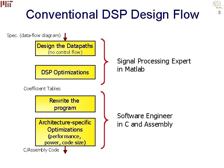
Conventional DSP Design Flow Spec. (data-flow diagram) Design the Datapaths (no control flow) DSP Optimizations Signal Processing Expert in Matlab Coefficient Tables Rewrite the program Architecture-specific Optimizations (performance, power, code size) C/Assembly Code Software Engineer in C and Assembly 3

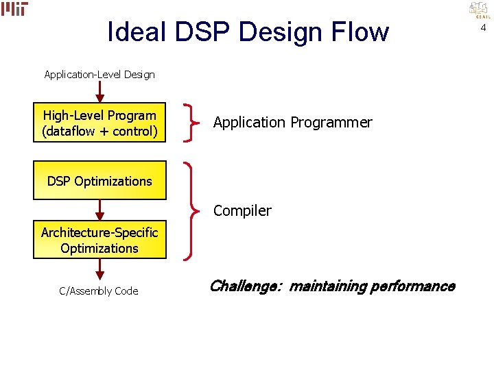
Ideal DSP Design Flow Application-Level Design High-Level Program (dataflow + control) Application Programmer DSP Optimizations Compiler Architecture-Specific Optimizations C/Assembly Code Challenge: maintaining performance 4

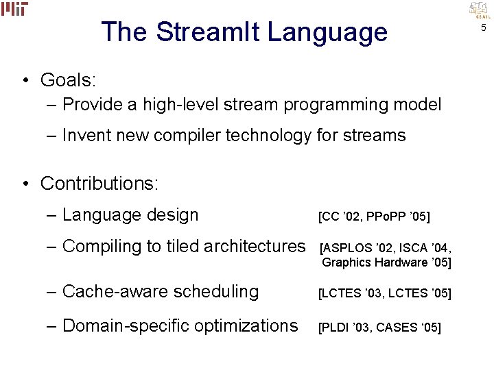
The Stream. It Language • Goals: – Provide a high-level stream programming model – Invent new compiler technology for streams • Contributions: – Language design [CC ’ 02, PPo. PP ’ 05] – Compiling to tiled architectures [ASPLOS ’ 02, ISCA ’ 04, Graphics Hardware ’ 05] – Cache-aware scheduling [LCTES ’ 03, LCTES ’ 05] – Domain-specific optimizations [PLDI ’ 03, CASES ‘ 05] 5

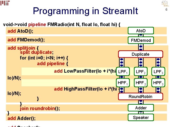
Programming in Stream. It void->void pipeline FMRadio(int N, float lo, float hi) { add Ato. D(); Ato. D add FMDemod(); FMDemod add splitjoin { split duplicate; for (int i=0; i<N; i++) { add pipeline { Duplicate add Low. Pass. Filter(lo + i*(hi -LPF 1 LPF 2 LPF 3 HPF 1 HPF 2 HPF 3 lo)/N); add High. Pass. Filter(lo + i*(hi } } join roundrobin(); } add Adder(); 6 Round. Robin Adder Speaker

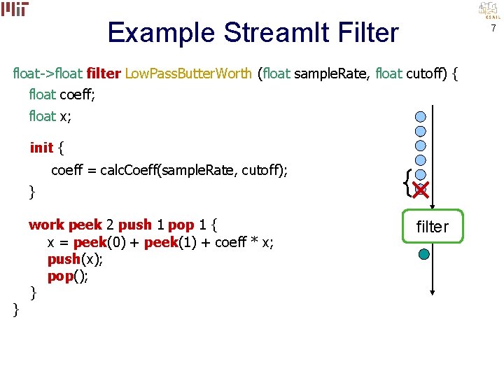
Example Stream. It Filter 7 float->float filter Low. Pass. Butter. Worth (float sample. Rate, float cutoff) { float coeff; float x; init { coeff = calc. Coeff(sample. Rate, cutoff); } } work peek 2 push 1 pop 1 { x = peek(0) + peek(1) + coeff * x; push(x); pop(); } filter

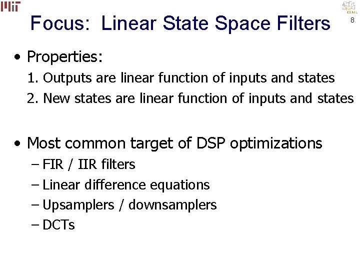
Focus: Linear State Space Filters 8 • Properties: 1. Outputs are linear function of inputs and states 2. New states are linear function of inputs and states • Most common target of DSP optimizations – FIR / IIR filters – Linear difference equations – Upsamplers / downsamplers – DCTs

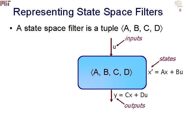
Representing State Space Filters 9 • A state space filter is a tuple A, B, C, D inputs u states A, B, C, D y = Cx + Du outputs x’ = Ax + Bu

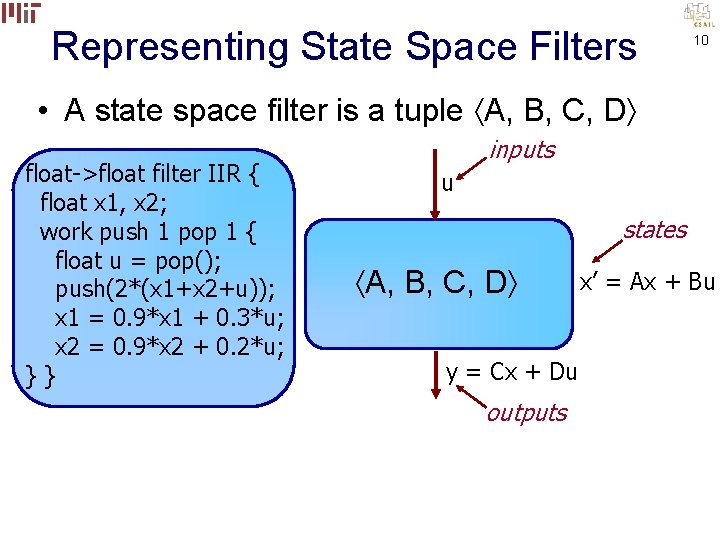
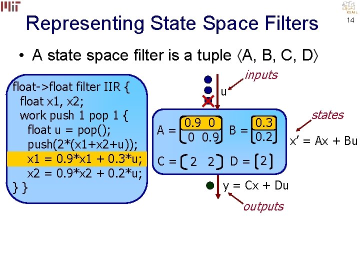
Representing State Space Filters 10 • A state space filter is a tuple A, B, C, D float->float filter IIR { float x 1, x 2; work push 1 pop 1 { float u = pop(); push(2*(x 1+x 2+u)); x 1 = 0. 9*x 1 + 0. 3*u; x 2 = 0. 9*x 2 + 0. 2*u; }} inputs u states A, B, C, D y = Cx + Du outputs x’ = Ax + Bu

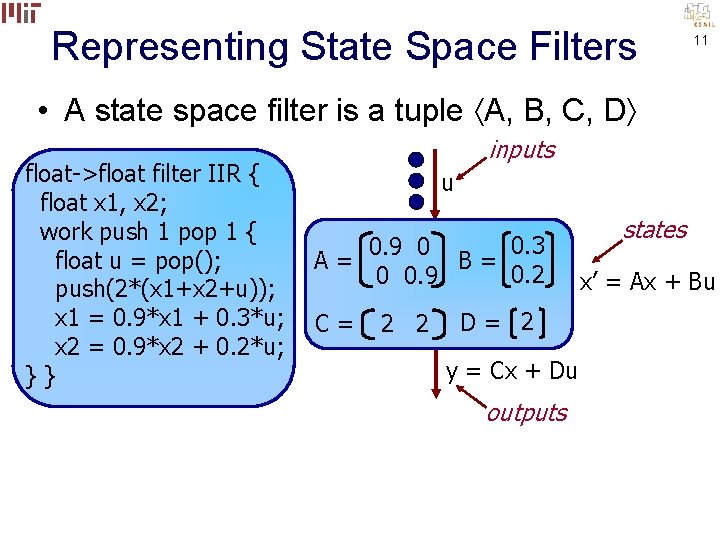
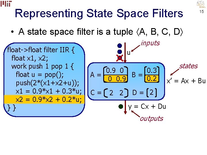
Representing State Space Filters 11 • A state space filter is a tuple A, B, C, D float->float filter IIR { float x 1, x 2; work push 1 pop 1 { float u = pop(); push(2*(x 1+x 2+u)); x 1 = 0. 9*x 1 + 0. 3*u; x 2 = 0. 9*x 2 + 0. 2*u; }} inputs u 0. 3 0. 9 0 A= B= 0. 2 0 0. 9 C= 2 2 D= 2 y = Cx + Du outputs states x’ = Ax + Bu

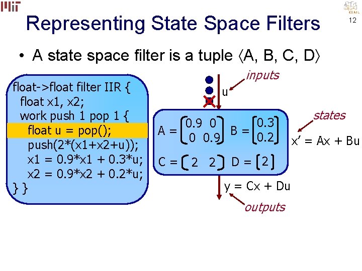
Representing State Space Filters 12 • A state space filter is a tuple A, B, C, D float->float filter IIR { float x 1, x 2; work push 1 pop 1 { float u = pop(); push(2*(x 1+x 2+u)); x 1 = 0. 9*x 1 + 0. 3*u; x 2 = 0. 9*x 2 + 0. 2*u; }} inputs u 0. 3 0. 9 0 A= B= 0. 2 0 0. 9 C= 2 2 D= 2 y = Cx + Du outputs states x’ = Ax + Bu

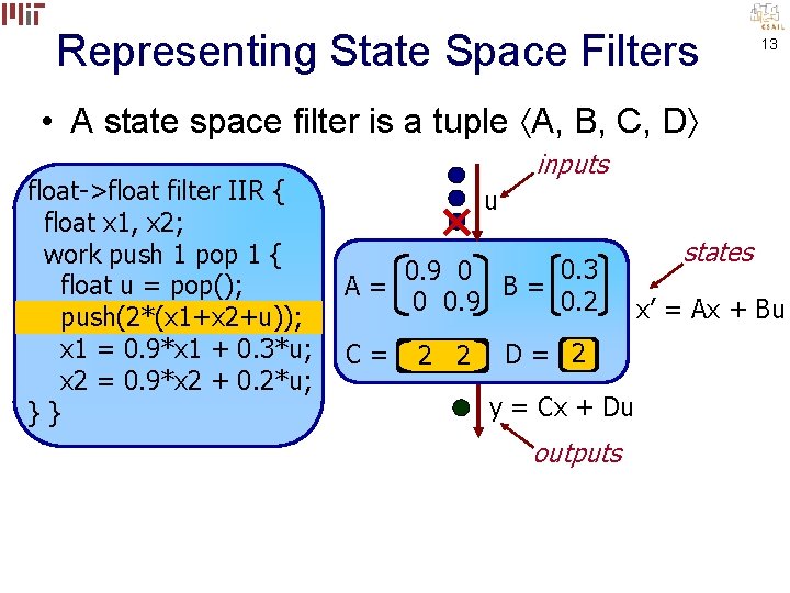
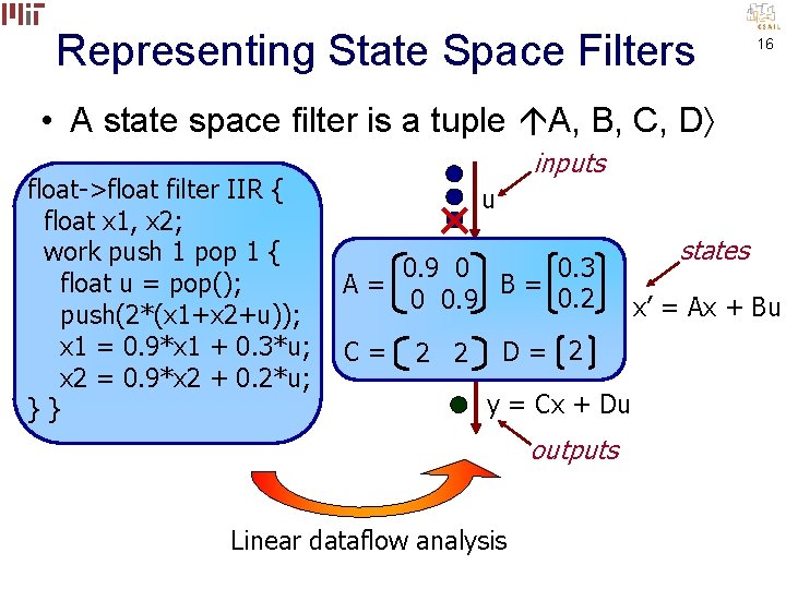
Representing State Space Filters 13 • A state space filter is a tuple A, B, C, D float->float filter IIR { float x 1, x 2; work push 1 pop 1 { float u = pop(); push(2*(x 1+x 2+u)); x 1 = 0. 9*x 1 + 0. 3*u; x 2 = 0. 9*x 2 + 0. 2*u; }} inputs u 0. 3 0. 9 0 A= B= 0. 2 0 0. 9 C= 2 2 D= 2 y = Cx + Du outputs states x’ = Ax + Bu

Representing State Space Filters 14 • A state space filter is a tuple A, B, C, D float->float filter IIR { float x 1, x 2; work push 1 pop 1 { float u = pop(); push(2*(x 1+x 2+u)); x 1 = 0. 9*x 1 + 0. 3*u; x 2 = 0. 9*x 2 + 0. 2*u; }} inputs u 0. 3 0. 9 0 A= B= 0. 2 0 0. 9 C= 2 2 D= 2 y = Cx + Du outputs states x’ = Ax + Bu

Representing State Space Filters 15 • A state space filter is a tuple A, B, C, D float->float filter IIR { float x 1, x 2; work push 1 pop 1 { float u = pop(); push(2*(x 1+x 2+u)); x 1 = 0. 9*x 1 + 0. 3*u; x 2 = 0. 9*x 2 + 0. 2*u; }} inputs u 0. 3 0. 9 0 A= B= 0. 2 0 0. 9 C= 2 2 D= 2 y = Cx + Du outputs states x’ = Ax + Bu

Representing State Space Filters 16 • A state space filter is a tuple A, B, C, D float->float filter IIR { float x 1, x 2; work push 1 pop 1 { float u = pop(); push(2*(x 1+x 2+u)); x 1 = 0. 9*x 1 + 0. 3*u; x 2 = 0. 9*x 2 + 0. 2*u; }} inputs u 0. 3 0. 9 0 A= B= 0. 2 0 0. 9 C= 2 2 D= 2 y = Cx + Du outputs Linear dataflow analysis states x’ = Ax + Bu

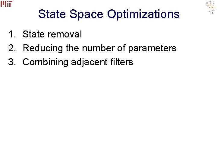
State Space Optimizations 1. State removal 2. Reducing the number of parameters 3. Combining adjacent filters 17

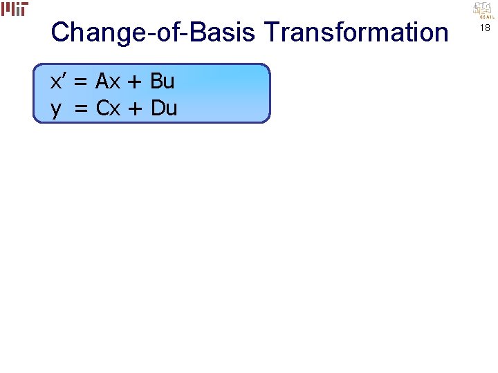
Change-of-Basis Transformation x’ = Ax + Bu y = Cx + Du 18

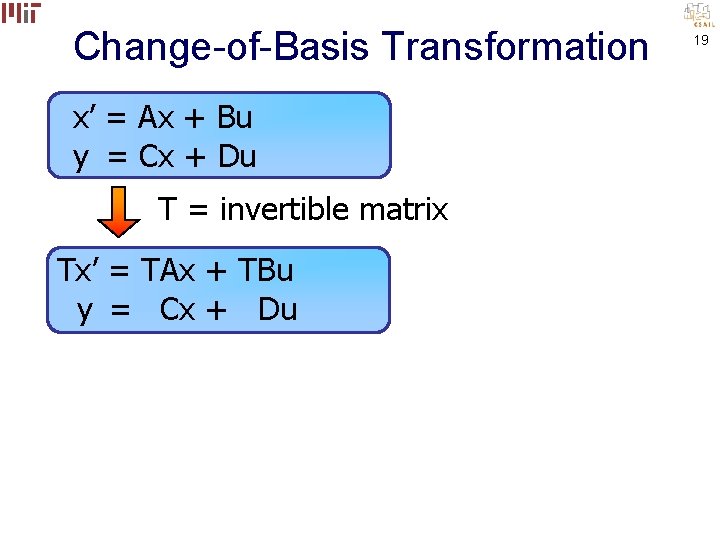
Change-of-Basis Transformation x’ = Ax + Bu y = Cx + Du T = invertible matrix Tx’ = TAx + TBu y = Cx + Du 19

Change-of-Basis Transformation x’ = Ax + Bu y = Cx + Du T = invertible matrix Tx’ = TA(T-1 T)x + TBu y = C(T-1 T)x + Du 20

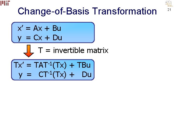
Change-of-Basis Transformation x’ = Ax + Bu y = Cx + Du T = invertible matrix Tx’ = TAT-1(Tx) + TBu y = CT-1(Tx) + Du 21

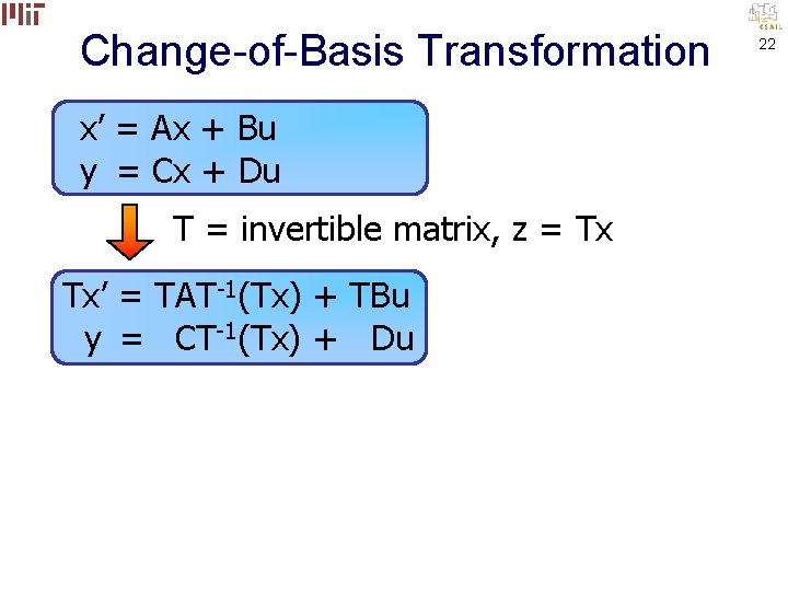
Change-of-Basis Transformation x’ = Ax + Bu y = Cx + Du T = invertible matrix, z = Tx Tx’ = TAT-1(Tx) + TBu y = CT-1(Tx) + Du 22

Change-of-Basis Transformation x’ = Ax + Bu y = Cx + Du T = invertible matrix, z = Tx z’ = TAT-1 z + TBu y = CT-1 z + Du 23

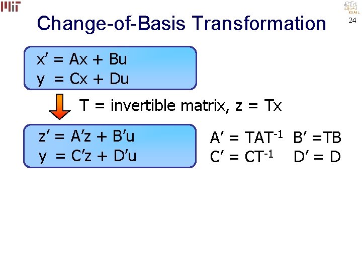
Change-of-Basis Transformation x’ = Ax + Bu y = Cx + Du T = invertible matrix, z = Tx z’ = A’z + B’u y = C’z + D’u A’ = TAT-1 B’ =TB C’ = CT-1 D’ = D 24

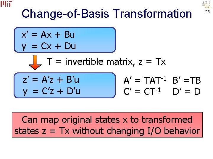
Change-of-Basis Transformation x’ = Ax + Bu y = Cx + Du T = invertible matrix, z = Tx z’ = A’z + B’u y = C’z + D’u A’ = TAT-1 B’ =TB C’ = CT-1 D’ = D Can map original states x to transformed states z = Tx without changing I/O behavior 25

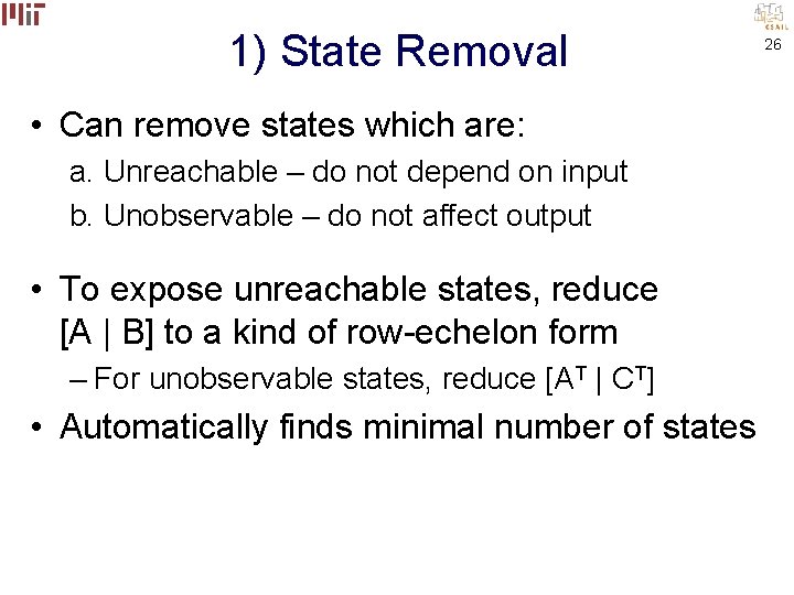
1) State Removal • Can remove states which are: a. Unreachable – do not depend on input b. Unobservable – do not affect output • To expose unreachable states, reduce [A | B] to a kind of row-echelon form – For unobservable states, reduce [AT | CT] • Automatically finds minimal number of states 26

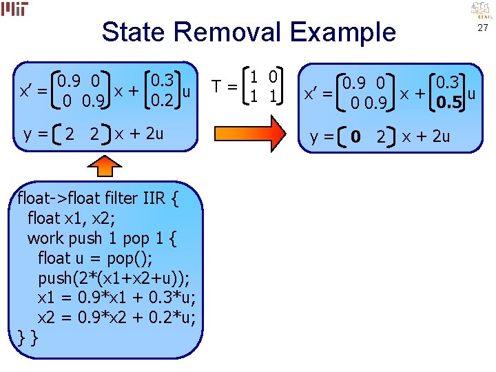
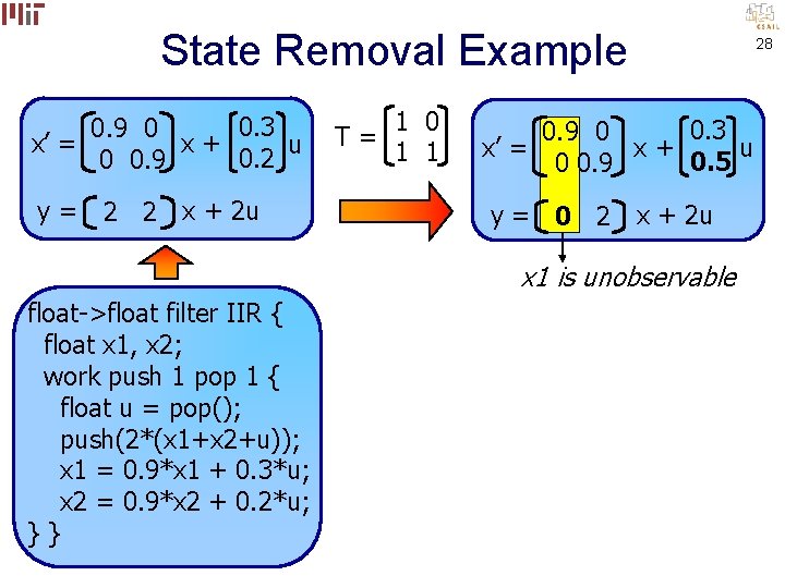
State Removal Example 0. 3 0. 9 0 x’ = x+ u 0. 2 0 0. 9 y= 2 2 x + 2 u float->float filter IIR { float x 1, x 2; work push 1 pop 1 { float u = pop(); push(2*(x 1+x 2+u)); x 1 = 0. 9*x 1 + 0. 3*u; x 2 = 0. 9*x 2 + 0. 2*u; }} 1 0 T= 1 1 x’ = 0. 3 0. 9 0 u x+ 0. 5 0 0. 9 y = 0 2 x + 2 u 27

State Removal Example 0. 3 0. 9 0 x’ = x+ u 0. 2 0 0. 9 y= 2 2 x + 2 u 1 0 T= 1 1 x’ = 0. 3 0. 9 0 u x+ 0. 5 0 0. 9 y = 0 2 x + 2 u x 1 is unobservable float->float filter IIR { float x 1, x 2; work push 1 pop 1 { float u = pop(); push(2*(x 1+x 2+u)); x 1 = 0. 9*x 1 + 0. 3*u; x 2 = 0. 9*x 2 + 0. 2*u; }} 28

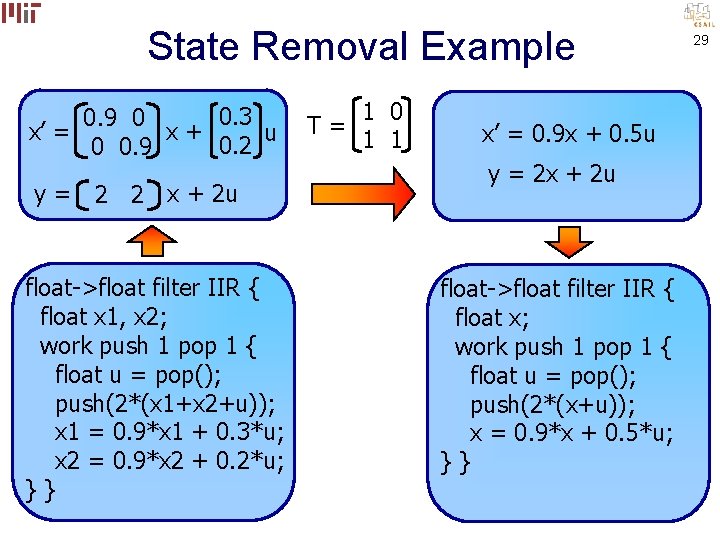
State Removal Example 0. 3 0. 9 0 x’ = x+ u 0. 2 0 0. 9 y= 2 2 x + 2 u float->float filter IIR { float x 1, x 2; work push 1 pop 1 { float u = pop(); push(2*(x 1+x 2+u)); x 1 = 0. 9*x 1 + 0. 3*u; x 2 = 0. 9*x 2 + 0. 2*u; }} 1 0 T= 1 1 x’ = 0. 9 x + 0. 5 u y = 2 x + 2 u float->float filter IIR { float x; work push 1 pop 1 { float u = pop(); push(2*(x+u)); x = 0. 9*x + 0. 5*u; }} 29

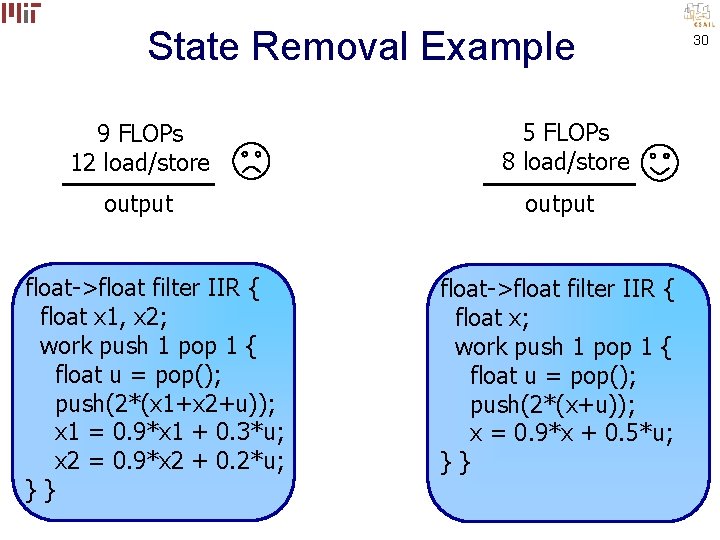
State Removal Example 9 FLOPs 12 load/store 5 FLOPs 8 load/store output float->float filter IIR { float x 1, x 2; work push 1 pop 1 { float u = pop(); push(2*(x 1+x 2+u)); x 1 = 0. 9*x 1 + 0. 3*u; x 2 = 0. 9*x 2 + 0. 2*u; }} float->float filter IIR { float x; work push 1 pop 1 { float u = pop(); push(2*(x+u)); x = 0. 9*x + 0. 5*u; }} 30

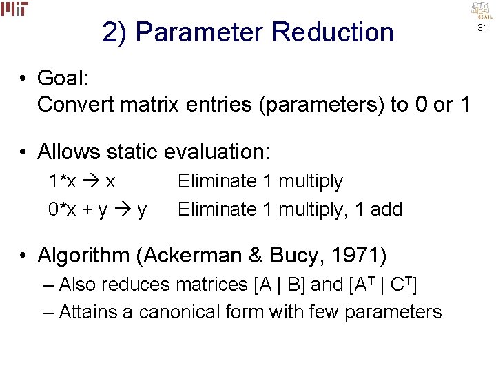
2) Parameter Reduction • Goal: Convert matrix entries (parameters) to 0 or 1 • Allows static evaluation: 1*x x 0*x + y y Eliminate 1 multiply, 1 add • Algorithm (Ackerman & Bucy, 1971) – Also reduces matrices [A | B] and [AT | CT] – Attains a canonical form with few parameters 31

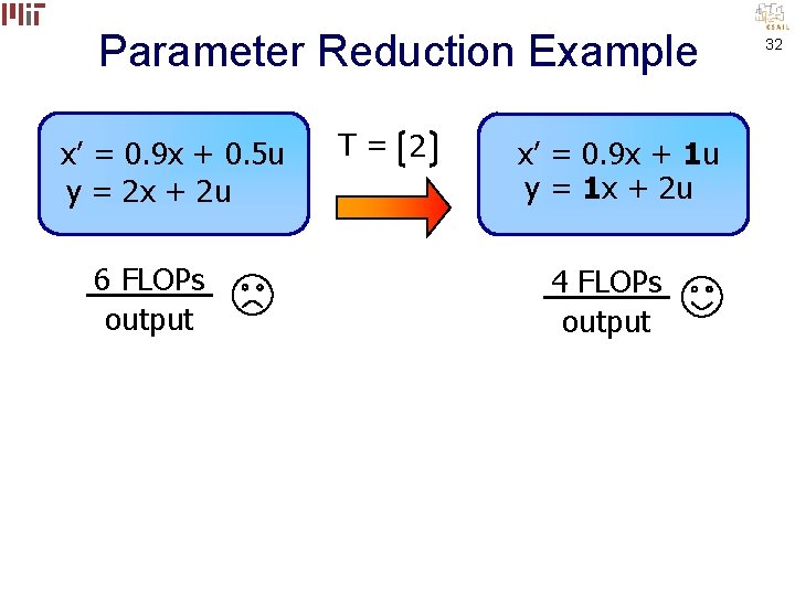
Parameter Reduction Example x’ = 0. 9 x + 0. 5 u y = 2 x + 2 u 6 FLOPs output T= 2 x’ = 0. 9 x + 1 u y = 1 x + 2 u 4 FLOPs output 32

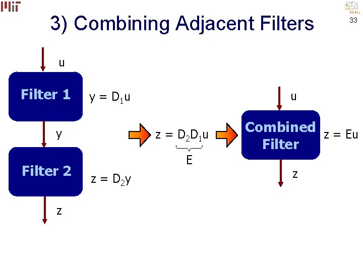
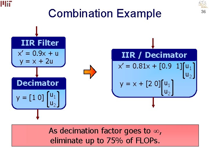
3) Combining Adjacent Filters 33 u Filter 1 y Filter 2 z u y = D 1 u z = D 2 D 1 u E z = D 2 y Combined z = Eu Filter z

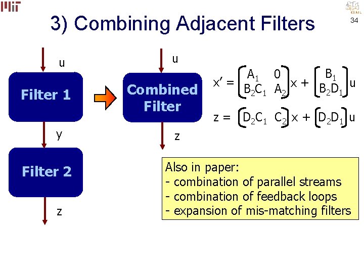
3) Combining Adjacent Filters u Filter 1 y Filter 2 z 34 u Combined Filter B 1 A 1 0 x’ = B 2 C 1 A 2 x + B 2 D 1 u z = D 2 C 1 C 2 x + D 2 D 1 u z Also in paper: - combination of parallel streams - combination of feedback loops - expansion of mis-matching filters

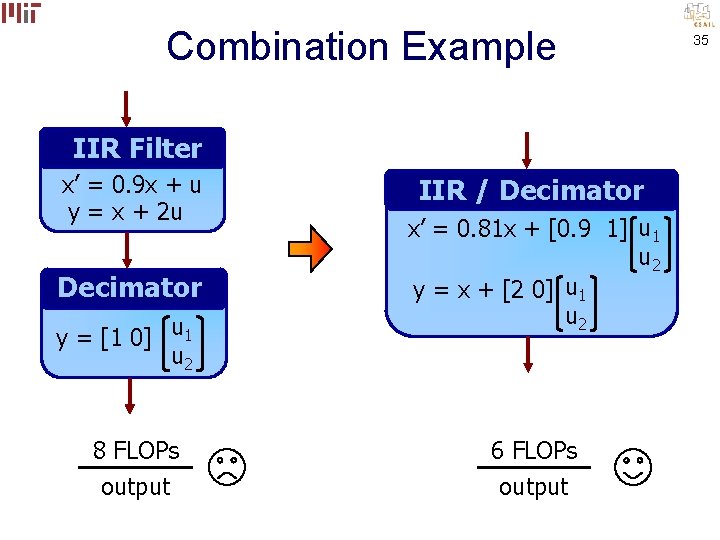
Combination Example IIR Filter x’ = 0. 9 x + u y = x + 2 u Decimator y = [1 0] u 1 u 2 8 FLOPs output IIR / Decimator x’ = 0. 81 x + [0. 9 1] u 1 u 2 y = x + [2 0] u 1 u 2 6 FLOPs output 35

Combination Example IIR Filter x’ = 0. 9 x + u y = x + 2 u Decimator y = [1 0] u 1 u 2 IIR / Decimator x’ = 0. 81 x + [0. 9 1] u 1 u 2 y = x + [2 0] u 1 u 2 8 FLOPs. As decimation factor goes 6 to. FLOPs , output eliminate up to 75% of FLOPs. 36

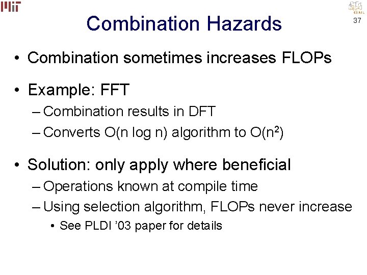
Combination Hazards • Combination sometimes increases FLOPs • Example: FFT – Combination results in DFT – Converts O(n log n) algorithm to O(n 2) • Solution: only apply where beneficial – Operations known at compile time – Using selection algorithm, FLOPs never increase • See PLDI ’ 03 paper for details 37

Results 38 • Subsumes combination of linear components – Evaluated previously [PLDI ’ 03] • Applications: FIR, Rate. Convert, Target. Detect, Radar, FMRadio, Filter. Bank, Vocoder, Oversampler, Dto. A – Removed 44% of FLOPs – Speedup of 120% on Pentium 4 • Results using state space analysis IIR + 1: 2 Decimator IIR + 1: 16 Decimator Speedup (Pentium 3) 49% 87%

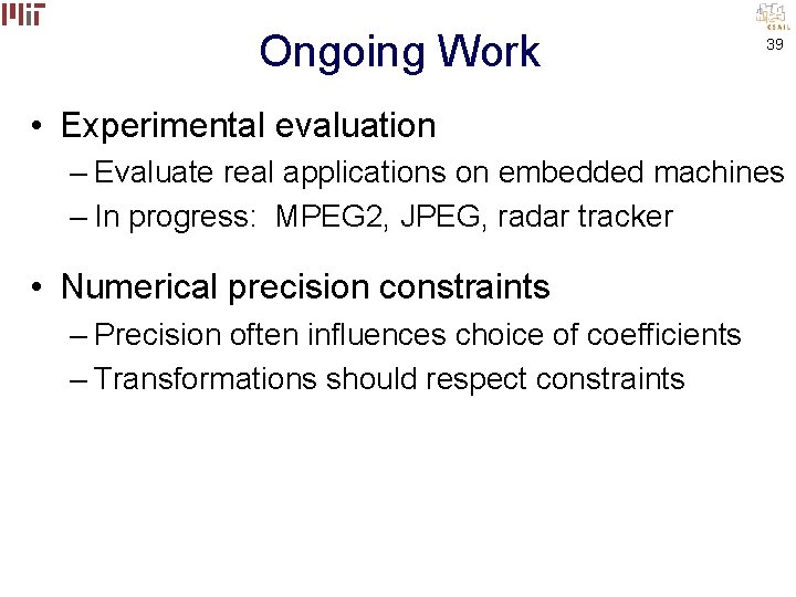
Ongoing Work 39 • Experimental evaluation – Evaluate real applications on embedded machines – In progress: MPEG 2, JPEG, radar tracker • Numerical precision constraints – Precision often influences choice of coefficients – Transformations should respect constraints

Related Work 40 • Linear stream optimizations [Lamb et al. ’ 03] – Deals with stateless filters • Automatic optimization of linear libraries – SPIRAL, FFTW, ATLAS, Sparsity • Stream languages – Lustre, Esterel, Signal, Lucid Synchrone, Brook, Spidle, Cg, Occam , Sisal, Parallel Haskell • Common sub-expression elimination

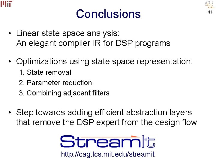
Conclusions • Linear state space analysis: An elegant compiler IR for DSP programs • Optimizations using state space representation: 1. State removal 2. Parameter reduction 3. Combining adjacent filters • Step towards adding efficient abstraction layers that remove the DSP expert from the design flow http: //cag. lcs. mit. edu/streamit 41