1 of 56 Chapter 21 The Simplest ShortRun

1 of 56 Chapter 21 The Simplest Short-Run Macro Model Copyright © 2011 Pearson Canada Inc.

2 of 56 In this chapter you will learn. . . 1. …the difference between desired expenditure and actual expenditure. 2. …the determinants of desired consumption and desired investment expenditures. 3. …the meaning of equilibrium national income. 4. …how a change in desired expenditure affects equilibrium income through the “simple multiplier. ” Copyright © 2011 Pearson Canada Inc.

3 of 56 21. 1 Desired Aggregate Expenditure The national accounts divide actual GDP into its components: - Ca, Ia , Ga, and NXa. Total desired expenditure is divided into the same categories: • desired consumption, C • desired investment, I • desired government purchases, G • desired net exports, NX Where are the ‘a’ subscripts? mfc 2007 mfc 2007 Copyright © 2011 Pearson Canada Inc.

4 of 56 National income accountants are interested in actual GDP and its components: Ca, Ia , Ga, and NXa. What actually occurred last period Macro Economic Theory is concerned with total desired expenditure and its components AE, C, I , G, NX Where are the ‘a’ subscripts? They are gone because we are referring to desired expenditure not actual! What do economic agents intend to do in the coming period? What plans have they made and how did they formulated those plans? MFC 2007 MFC 2007

5 of 56 The sum is called desired aggregate expenditure: AE = C + I + G + NX Where are the ‘a’ subscripts? You absolutely need to understand why the subscripts ‘a’ are not in the AE expression! mfc 2007 mfc 2007 Copyright © 2011 Pearson Canada Inc.

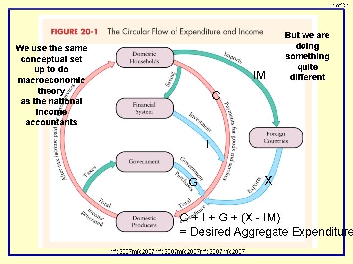
6 of 56 We use the same conceptual set up to do macroeconomic theory as the national income accountants IM But we are doing something quite different C I G X C + I + G + (X - IM) = Desired Aggregate Expenditure mfc 2007 mfc 2007

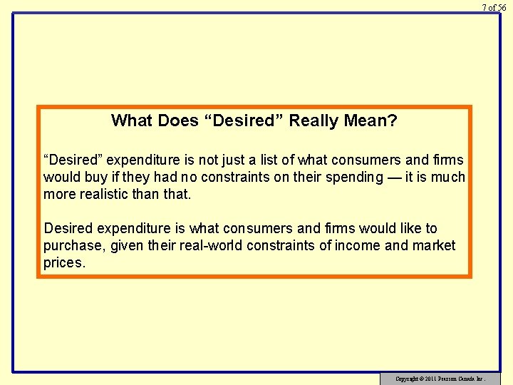
7 of 56 What Does “Desired” Really Mean? “Desired” expenditure is not just a list of what consumers and firms would buy if they had no constraints on their spending — it is much more realistic than that. Desired expenditure is what consumers and firms would like to purchase, given their real-world constraints of income and market prices. Copyright © 2011 Pearson Canada Inc.

8 of 56 Two general types of expenditures: - autonomous expenditures do not depend on the level of national income - induced expenditures do depend on the level of national income MFC 2007 MFC 2007

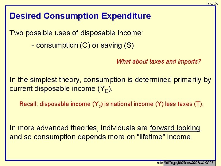
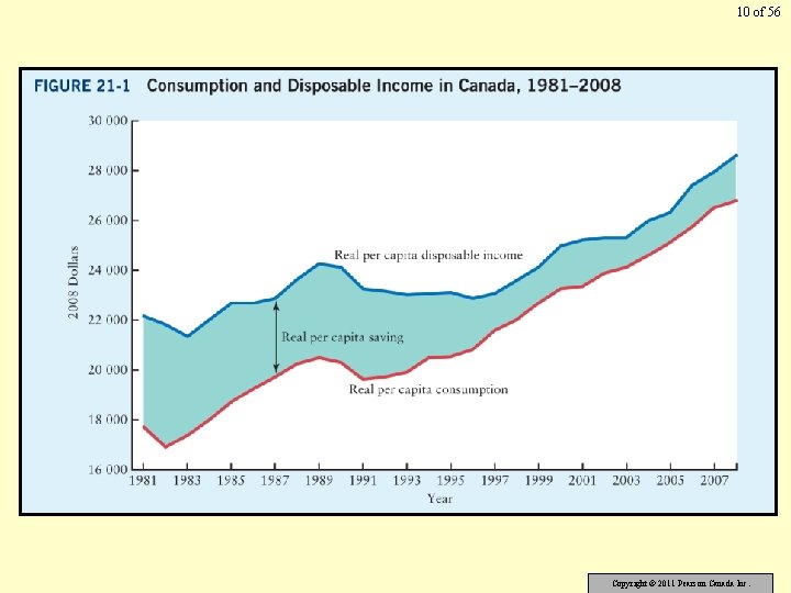
9 of 56 Desired Consumption Expenditure Two possible uses of disposable income: - consumption (C) or saving (S) What about taxes and imports? In the simplest theory, consumption is determined primarily by current disposable income (YD). Recall: disposable income (Yd) is national income (Y) less taxes (T). In more advanced theories, individuals are forward looking, and so consumption depends more on “lifetime” income. mfc 2007 mfc 2007 Copyright © 2011 Pearson Canada Inc.

10 of 56 Copyright © 2011 Pearson Canada Inc.

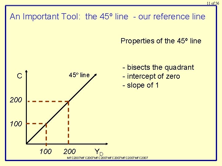
11 of 56 An Important Tool: the 45º line - our reference line Properties of the 45º line - bisects the quadrant - intercept of zero - slope of 1 45º line C 200 100 200 YD MFC 2007 MFC 2007

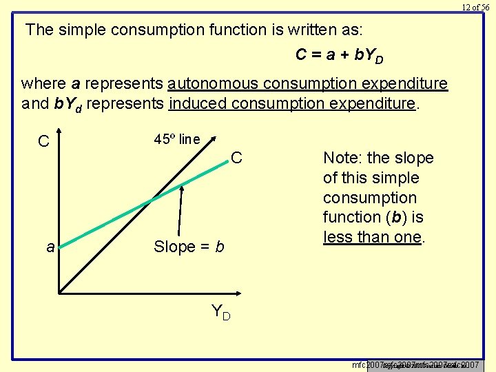
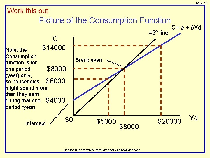
12 of 56 The simple consumption function is written as: C = a + b. YD where a represents autonomous consumption expenditure and b. Yd represents induced consumption expenditure. C a 45º line C Slope = b Note: the slope of this simple consumption function (b) is less than one. YD mfc 2007 mfc 2007 Copyright © 2011 Pearson Canada Inc.

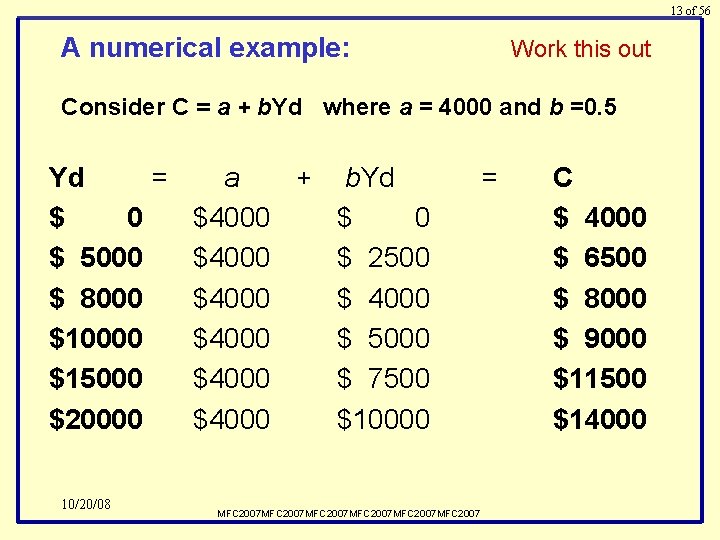
13 of 56 A numerical example: Work this out Consider C = a + b. Yd where a = 4000 and b =0. 5 Yd = a + b. Yd $ 0 $4000 $ 5000 $4000 $ 2500 $ 8000 $4000 $10000 $4000 $ 5000 $15000 $4000 $ 7500 $20000 $4000 $10000 10/20/08 MFC 2007 MFC 2007 = C $ 4000 $ 6500 $ 8000 $ 9000 $11500 $14000

14 of 56 Work this out Picture of the Consumption Function 45º line C $14000 Note: the Consumption function is for one period $8000 (year) only, so households $6000 might spend more than they earn during that one $4000 period (year) Intercept $0 C= a + b. Yd Break even $5000 $8000 MFC 2007 MFC 2007 $20000 Yd

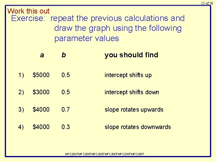
15 of 56 Work this out Exercise: repeat the previous calculations and draw the graph using the following parameter values a b you should find 1) $5000 0. 5 intercept shifts up 2) $3000 0. 5 intercept shifts down 3) $4000 0. 7 slope rotates upwards 4) $4000 0. 3 slope rotates downwards MFC 2007 MFC 2007

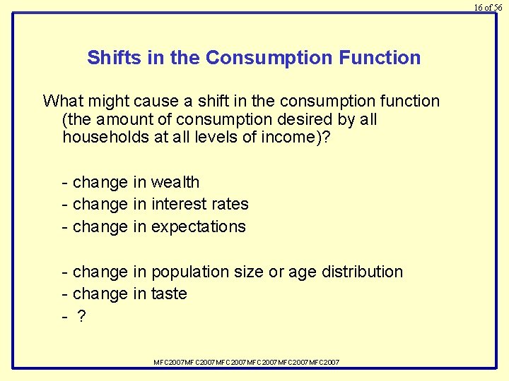
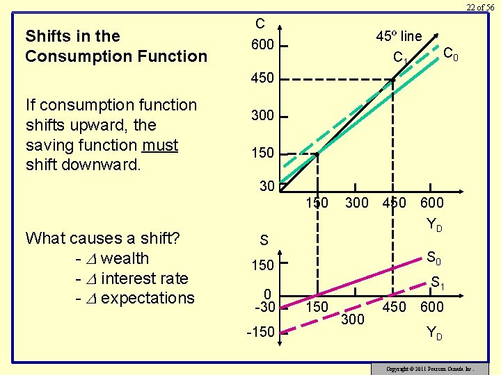
16 of 56 Shifts in the Consumption Function What might cause a shift in the consumption function (the amount of consumption desired by all households at all levels of income)? - change in wealth - change in interest rates - change in expectations - change in population size or age distribution - change in taste - ? MFC 2007 MFC 2007

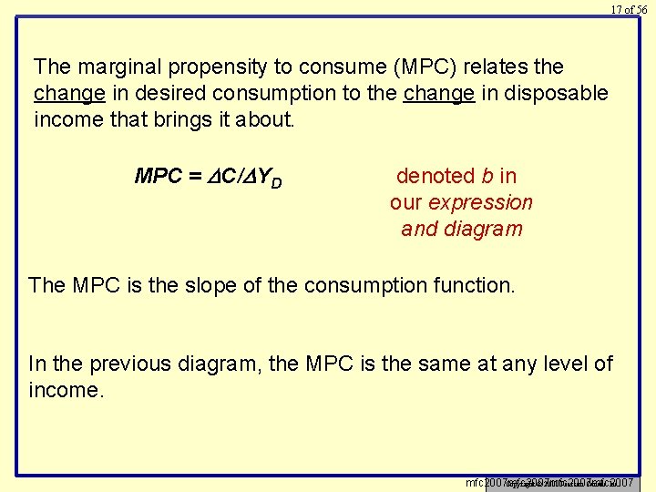
17 of 56 The marginal propensity to consume (MPC) relates the change in desired consumption to the change in disposable income that brings it about. MPC = C/ YD denoted b in our expression and diagram The MPC is the slope of the consumption function. In the previous diagram, the MPC is the same at any level of income. mfc 2007 mfc 2007 Copyright © 2011 Pearson Canada Inc.

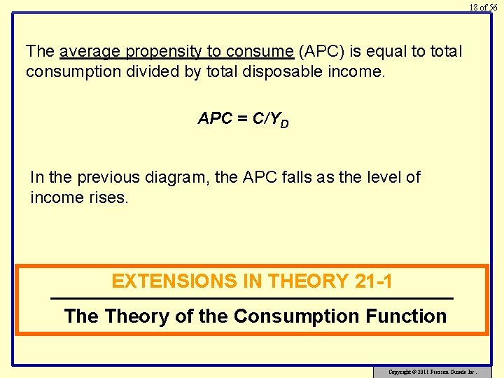
18 of 56 The average propensity to consume (APC) is equal to total consumption divided by total disposable income. APC = C/YD In the previous diagram, the APC falls as the level of income rises. EXTENSIONS IN THEORY 21 -1 Theory of the Consumption Function Copyright © 2011 Pearson Canada Inc.

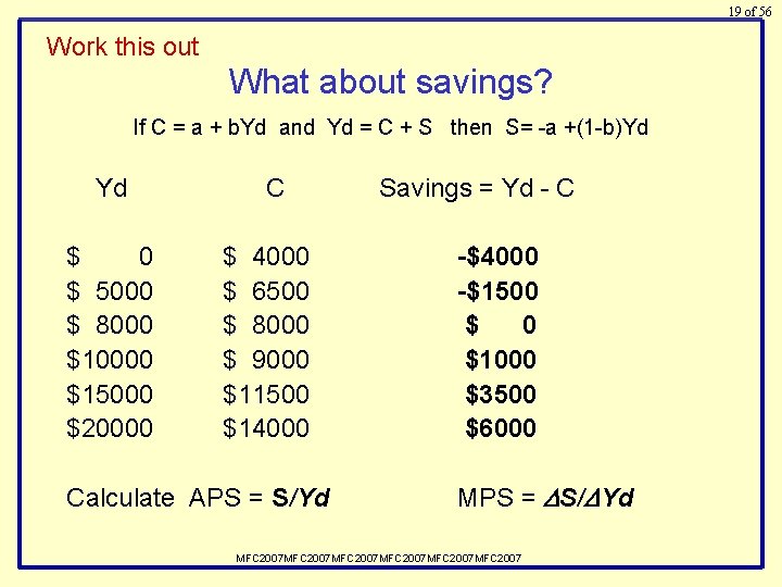
19 of 56 Work this out What about savings? If C = a + b. Yd and Yd = C + S then S= -a +(1 -b)Yd Yd $ 0 $ 5000 $ 8000 $10000 $15000 $20000 C $ 4000 $ 6500 $ 8000 $ 9000 $11500 $14000 Calculate APS = S/Yd Savings = Yd - C -$4000 -$1500 $ 0 $1000 $3500 $6000 MPS = S/ Yd MFC 2007 MFC 2007

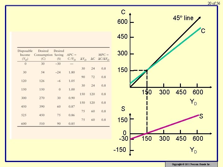
20 of 56 C 45º line 600 C 450 300 150 • 150 300 450 S 600 YD S 150 0 -30 -150 300 450 600 YD Copyright © 2011 Pearson Canada Inc.

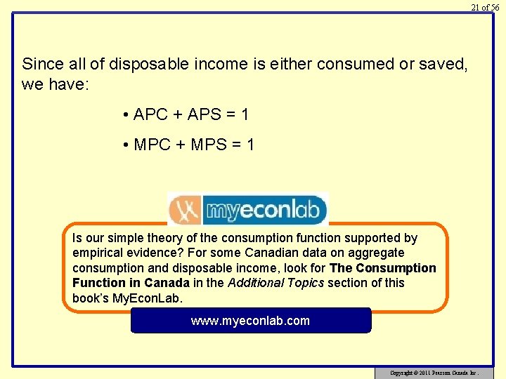
21 of 56 Since all of disposable income is either consumed or saved, we have: • APC + APS = 1 • MPC + MPS = 1 Is our simple theory of the consumption function supported by empirical evidence? For some Canadian data on aggregate consumption and disposable income, look for The Consumption Function in Canada in the Additional Topics section of this book’s My. Econ. Lab. www. myeconlab. com Copyright © 2011 Pearson Canada Inc.

22 of 56 Shifts in the Consumption Function C 600 45º line C 1 450 If consumption function shifts upward, the saving function must shift downward. C 0 • 300 150 • 30 150 What causes a shift? - wealth - interest rate - expectations 300 450 S S 0 150 0 -30 -150 600 YD S 1 150 300 450 600 YD Copyright © 2011 Pearson Canada Inc.

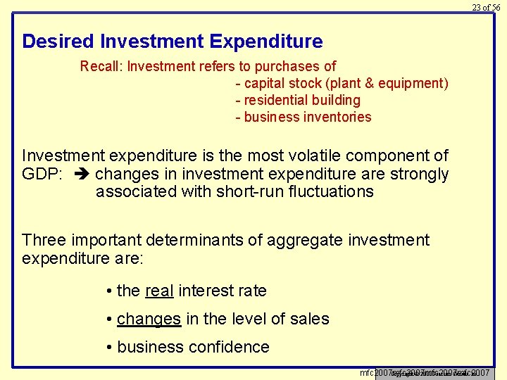
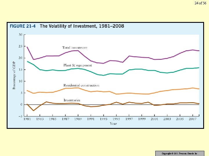
23 of 56 Desired Investment Expenditure Recall: Investment refers to purchases of - capital stock (plant & equipment) - residential building - business inventories Investment expenditure is the most volatile component of GDP: changes in investment expenditure are strongly associated with short-run fluctuations Three important determinants of aggregate investment expenditure are: • the real interest rate • changes in the level of sales • business confidence mfc 2007 mfc 2007 Copyright © 2011 Pearson Canada Inc.

24 of 56 Copyright © 2011 Pearson Canada Inc.

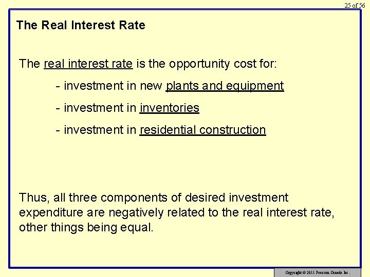
25 of 56 The Real Interest Rate The real interest rate is the opportunity cost for: - investment in new plants and equipment - investment in inventories - investment in residential construction Thus, all three components of desired investment expenditure are negatively related to the real interest rate, other things being equal. Copyright © 2011 Pearson Canada Inc.

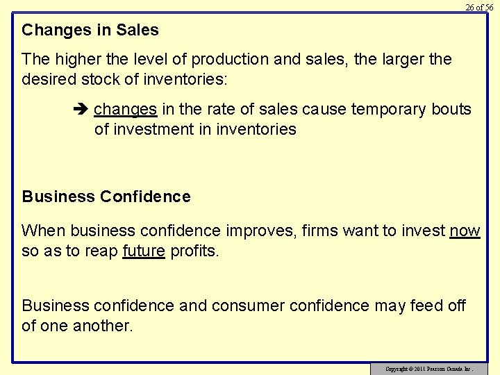
26 of 56 Changes in Sales The higher the level of production and sales, the larger the desired stock of inventories: changes in the rate of sales cause temporary bouts of investment in inventories Business Confidence When business confidence improves, firms want to invest now so as to reap future profits. Business confidence and consumer confidence may feed off of one another. Copyright © 2011 Pearson Canada Inc.

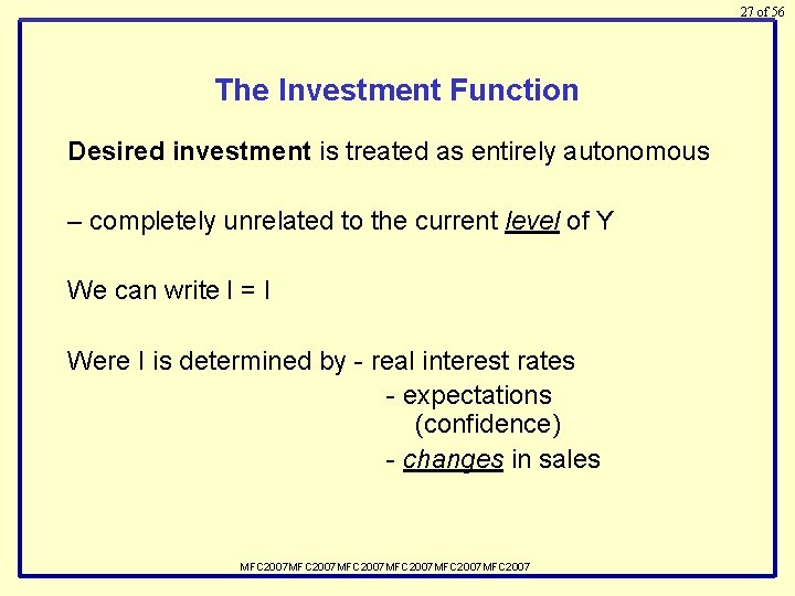
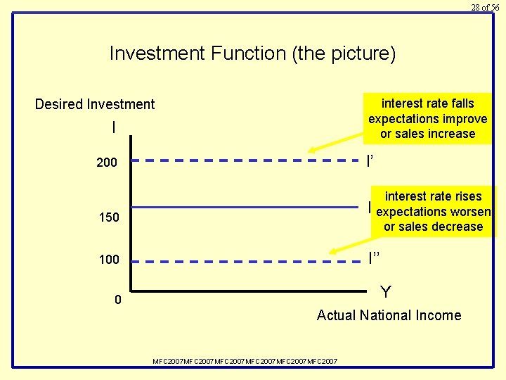
27 of 56 The Investment Function Desired investment is treated as entirely autonomous – completely unrelated to the current level of Y We can write I = I Were I is determined by - real interest rates - expectations (confidence) - changes in sales MFC 2007 MFC 2007

28 of 56 Investment Function (the picture) interest rate falls expectations improve or sales increase Desired Investment I 200 I’ 150 interest rate rises I expectations worsen or sales decrease 100 I’’ Y 0 Actual National Income MFC 2007 MFC 2007

29 of 56 Our Story – a simplified version (no Government, no Trade) We will now start to tell our story (assemble our macroeconomic model). Our story has two key purposes: - to explain what determines the level of aggregate economic activity (the size of the GDP or Y) - to understand what might cause GDP (Y) to increase and what might cause GDP (Y) to decrease? MFC 2007 MFC 2007

30 of 56 The Aggregate Expenditure Function The AE function: - relates desired aggregate expenditure to actual national income In the absence of government and international trade, desired aggregate expenditure is: AE = C + I This is called a ‘closed economy with no government’ no Government, no Trade AE = C + I + G + NX A Lou Dobbs economy (or perhaps the Fox Network economy). mfc 2007 mfc 2007 Copyright © 2011 Pearson Canada Inc.

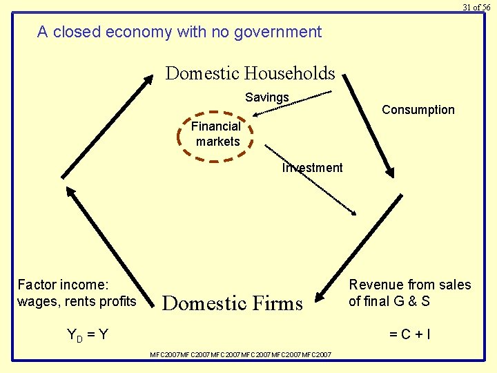
31 of 56 A closed economy with no government Domestic Households Savings Consumption Financial markets Investment Factor income: wages, rents profits Domestic Firms YD = Y Revenue from sales of final G & S =C+I MFC 2007 MFC 2007

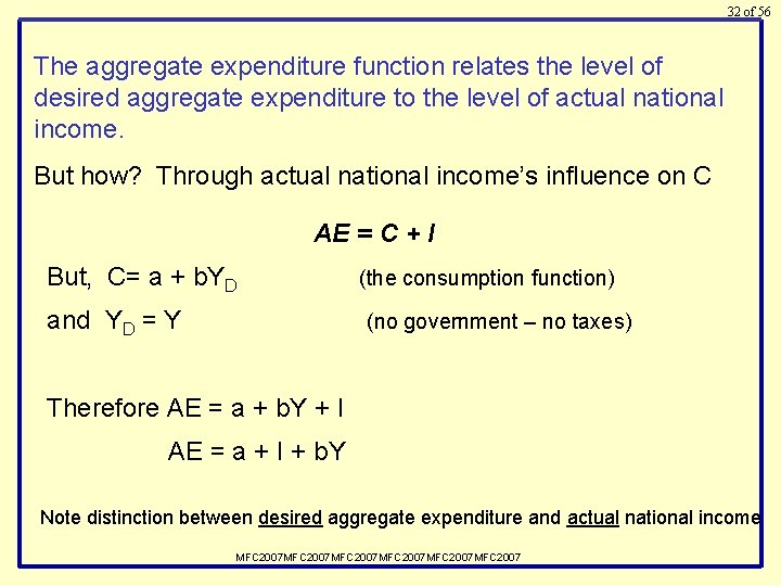
32 of 56 The aggregate expenditure function relates the level of desired aggregate expenditure to the level of actual national income. But how? Through actual national income’s influence on C AE = C + I But, C= a + b. YD and YD = Y (the consumption function) (no government – no taxes) Therefore AE = a + b. Y + I AE = a + I + b. Y Note distinction between desired aggregate expenditure and actual national income MFC 2007 MFC 2007

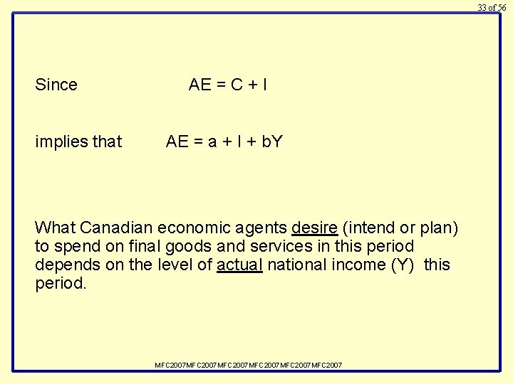
33 of 56 Since implies that AE = C + I AE = a + I + b. Y What Canadian economic agents desire (intend or plan) to spend on final goods and services in this period depends on the level of actual national income (Y) this period. MFC 2007 MFC 2007

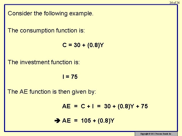
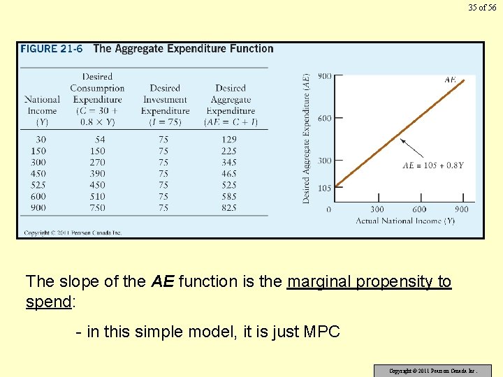
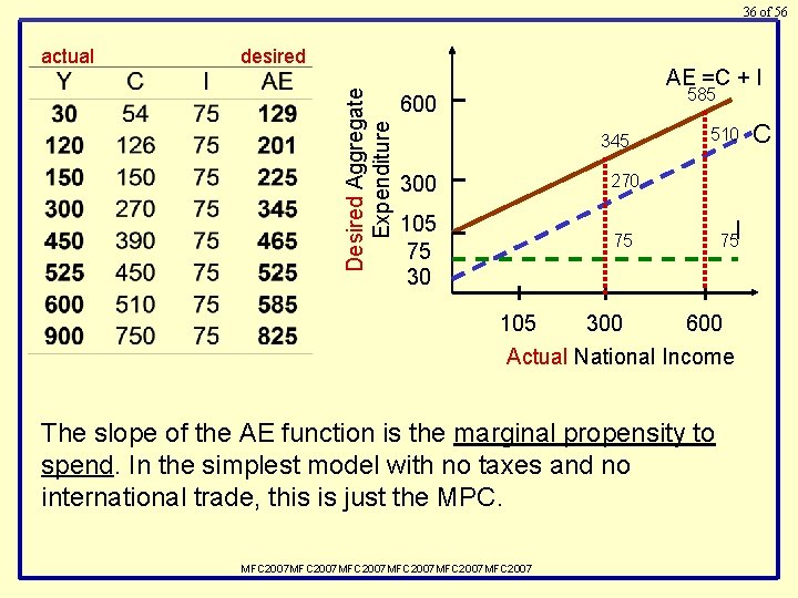
34 of 56 Consider the following example. The consumption function is: C = 30 + (0. 8)Y The investment function is: I = 75 The AE function is then given by: AE = C + I = 30 + (0. 8)Y + 75 AE = 105 + (0. 8)Y Copyright © 2011 Pearson Canada Inc.

35 of 56 The slope of the AE function is the marginal propensity to spend: - in this simple model, it is just MPC Copyright © 2011 Pearson Canada Inc.

36 of 56 desired Desired Aggregate Expenditure actual AE =C + I 585 600 345 510 270 300 105 75 30 75 75 I 105 300 600 Actual National Income The slope of the AE function is the marginal propensity to spend. In the simplest model with no taxes and no international trade, this is just the MPC. MFC 2007 MFC 2007 C

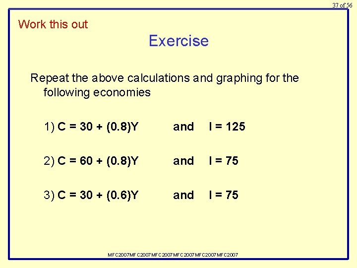
37 of 56 Work this out Exercise Repeat the above calculations and graphing for the following economies 1) C = 30 + (0. 8)Y and I = 125 2) C = 60 + (0. 8)Y and I = 75 3) C = 30 + (0. 6)Y and I = 75 MFC 2007 MFC 2007

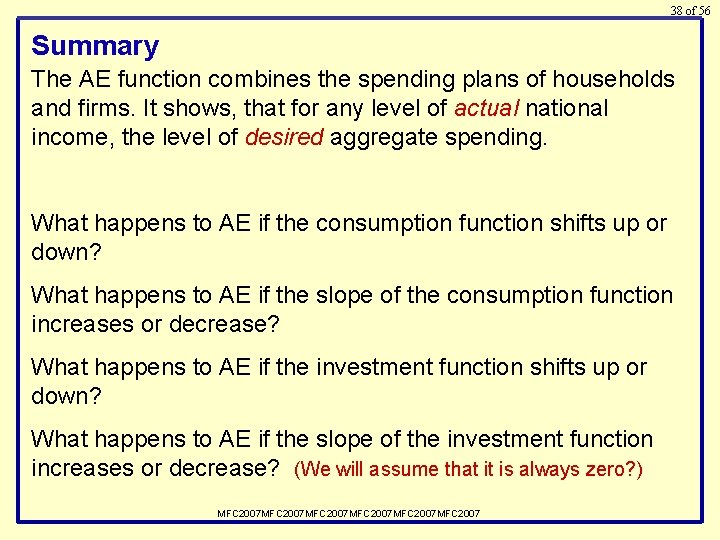
38 of 56 Summary The AE function combines the spending plans of households and firms. It shows, that for any level of actual national income, the level of desired aggregate spending. What happens to AE if the consumption function shifts up or down? What happens to AE if the slope of the consumption function increases or decrease? What happens to AE if the investment function shifts up or down? What happens to AE if the slope of the investment function increases or decrease? (We will assume that it is always zero? ) MFC 2007 MFC 2007

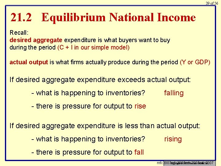
39 of 56 21. 2 Equilibrium National Income Recall: desired aggregate expenditure is what buyers want to buy during the period (C + I in our simple model) actual output is what firms actually produce during the period (Y or GDP) If desired aggregate expenditure exceeds actual output: - what is happening to inventories? falling - there is pressure for output to rise If desired aggregate expenditure is less than actual output: - what is happening to inventories? rising - there is pressure for output to fall mfc 2007 mfc 2007 Copyright © 2011 Pearson Canada Inc.

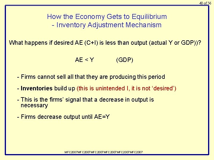
40 of 56 How the Economy Gets to Equilibrium - Inventory Adjustment Mechanism What happens if desired AE (C+I) is less than output (actual Y or GDP))? AE < Y (GDP) - Firms cannot sell all that they are producing this period - Inventories build up (this is unintended I, it is not ‘desired’) - This is the firms’ signal that a decrease in output is necessary - Firms decrease output until AE=Y MFC 2007 MFC 2007

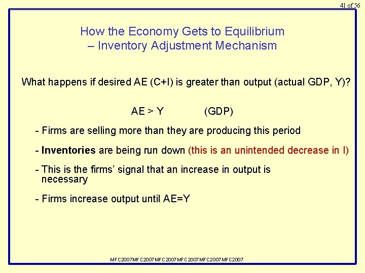
41 of 56 How the Economy Gets to Equilibrium – Inventory Adjustment Mechanism What happens if desired AE (C+I) is greater than output (actual GDP, Y)? AE > Y (GDP) - Firms are selling more than they are producing this period - Inventories are being run down (this is an unintended decrease in I) - This is the firms’ signal that an increase in output is necessary - Firms increase output until AE=Y MFC 2007 MFC 2007

42 of 56 Copyright © 2011 Pearson Canada Inc.

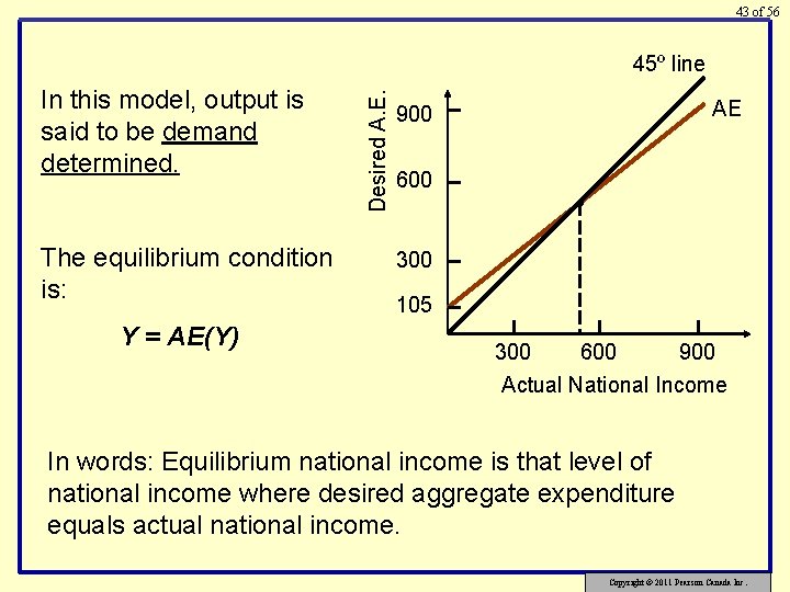
43 of 56 In this model, output is said to be demand determined. The equilibrium condition is: Y = AE(Y) Desired A. E. 45º line AE 900 600 • 300 105 300 600 900 Actual National Income In words: Equilibrium national income is that level of national income where desired aggregate expenditure equals actual national income. Copyright © 2011 Pearson Canada Inc.

44 of 56 Remember! INVENTORIES! MFC 2007 MFC 2007

45 of 56 A different, but equivalent, way of thinking about the equilibrium level of national income involves comparing desired saving with desired investment. For more details, look for Investment, Saving, and Equilibrium GDP in the Additional Topics section of this book’s My. Econ. Lab. www. myeconlab. com Copyright © 2011 Pearson Canada Inc.

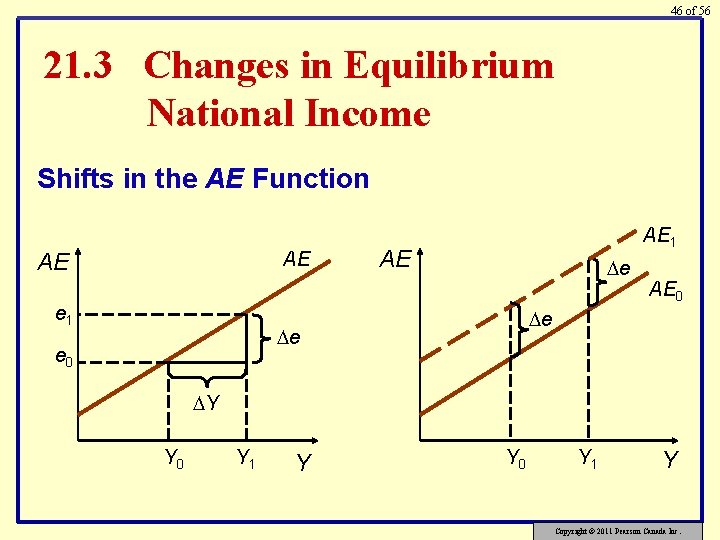
46 of 56 21. 3 Changes in Equilibrium National Income Shifts in the AE Function AE AE e 1 AE e e 0 AE 0 Y Y 0 Y 1 Y Copyright © 2011 Pearson Canada Inc.

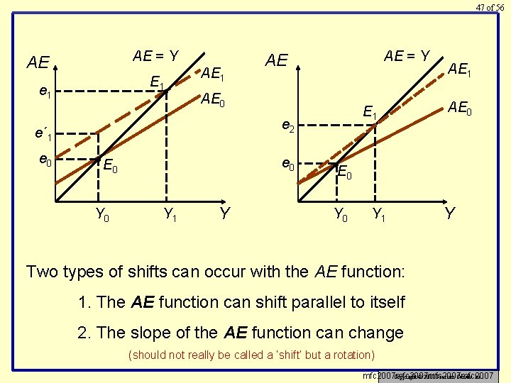
47 of 56 AE = Y AE E 1 e 1 • AE 1 AE 0 E 1 e 2 e´ 1 e 0 AE = Y AE • E 0 Y 0 e 0 Y 1 Y • • E AE 1 AE 0 0 Y 1 Y Two types of shifts can occur with the AE function: 1. The AE function can shift parallel to itself 2. The slope of the AE function can change (should not really be called a ‘shift’ but a rotation) mfc 2007 mfc 2007 Copyright © 2011 Pearson Canada Inc.

48 of 56 The Multiplier The multiplier is a measure of the size of the change in equilibrium Y that results from a change in autonomous expenditure. In our simplest of macro models, the multiplier exceeds one. APPLYING ECONOMIC CONCEPTS 21 -1 The Multiplier: A Numerical Example Copyright © 2011 Pearson Canada Inc.

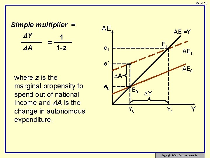
49 of 56 Simple multiplier = Y 1 = A 1 -z AE AE =Y E 1 e 1 • e´ 1 where z is the marginal propensity to spend out of national income and A is the change in autonomous expenditure. • AE 0 A e 0 • E Y 0 AE 1 0 Y Y 1 Y Copyright © 2011 Pearson Canada Inc.

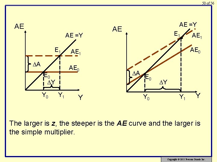
50 of 56 AE AE =Y E 1 • A • E 0 Y Y 1 AE E 1 • Y AE 1 AE 0 Y 0 AE =Y A • E 0 Y 0 Y Y 1 Y The larger is z, the steeper is the AE curve and the larger is the simple multiplier. Copyright © 2011 Pearson Canada Inc.

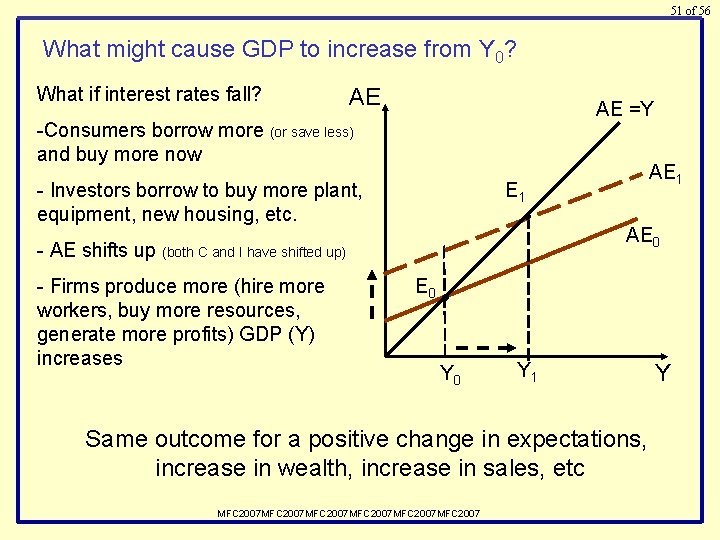
51 of 56 What might cause GDP to increase from Y 0? What if interest rates fall? AE AE =Y -Consumers borrow more (or save less) and buy more now - Investors borrow to buy more plant, equipment, new housing, etc. E 1 • - AE shifts up (both C and I have shifted up) - Firms produce more (hire more workers, buy more resources, generate more profits) GDP (Y) increases AE 1 E 0 AE 0 • Y 0 Y 1 Same outcome for a positive change in expectations, increase in wealth, increase in sales, etc MFC 2007 MFC 2007 Y

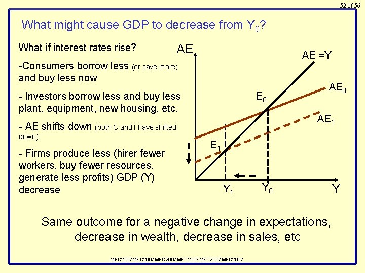
52 of 56 What might cause GDP to decrease from Y 0? What if interest rates rise? AE AE =Y -Consumers borrow less (or save more) and buy less now - Investors borrow less and buy less plant, equipment, new housing, etc. E 0 • - AE shifts down (both C and I have shifted down) - Firms produce less (hirer fewer workers, buy fewer resources, generate less profits) GDP (Y) decrease E 1 AE 0 AE 1 • Y 1 Y 0 Same outcome for a negative change in expectations, decrease in wealth, decrease in sales, etc MFC 2007 MFC 2007 Y

53 of 56 EXTENSIONS IN THEORY 21 -2 The Algebra of the Simple Multiplier Economic Fluctuations as Self-Fulfilling Prophecies Households and firms base their desired investment and consumption partly on their expectations of the future: changes in expectations can lead to real changes in the current state of the economy Copyright © 2011 Pearson Canada Inc.

54 of 56 Example: - imagine that firms feel optimistic about the future - this increases their desired investment, shifting up the AE curve - this increases Y, justifying the initial optimism Copyright © 2011 Pearson Canada Inc.

55 of 56 Now imagine the opposite scenario. It should be clear that if firms and households are pessimistic about the future in large numbers, the ensuing change in their behaviour will lead to a self-fulfilling prophecy of reduced national income. Could the Prime Minister (or the Governor of the Bank of Canada) ever announce to the country that they might have made a ‘big’ mistake? For example: suppose that government analysts report to the Prime Minister that having signed the Kyoto Accord might result in a recession. MFC 2007 MFC 2007

56 of 56 Copyright © 2011 Pearson Canada Inc.