1 Nominal Measures of Association 2 Ordinal Measure

1. Nominal Measures of Association 2. Ordinal Measure s of Associaiton

ASSOCIATION • Association – The strength of relationship between 2 variables – Knowing how much variables are related may enable you to predict the value of 1 variable when you know the value of another • As with test statistics, the proper measure of association depends on how variables are measured

Significance vs. Strength • Test statistics do (in a sense) capture the strength of a relationship – t = number of standard errors that separate means – Chi-Square = how different our findings are from what is expected under null • If null is no relationship, then higher Chi-square values indicate stronger relationships. • HOWEVER --- test statistics are also influenced by other stuff (e. g. , sample size)

MEASURES OF ASSOCIATION FOR NOMINALLEVEL VARIABLES “Chi-Square Based” Measures • Use 2, but remove influence of N – Phi – Cramer's V

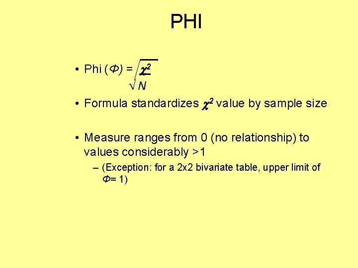
PHI • Phi (Φ) = 2 √N • Formula standardizes 2 value by sample size • Measure ranges from 0 (no relationship) to values considerably >1 – (Exception: for a 2 x 2 bivariate table, upper limit of Φ= 1)

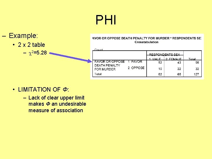
PHI – Example: • 2 x 2 table – 2=5. 28 • LIMITATION OF Φ: – Lack of clear upper limit makes Φ an undesirable measure of association

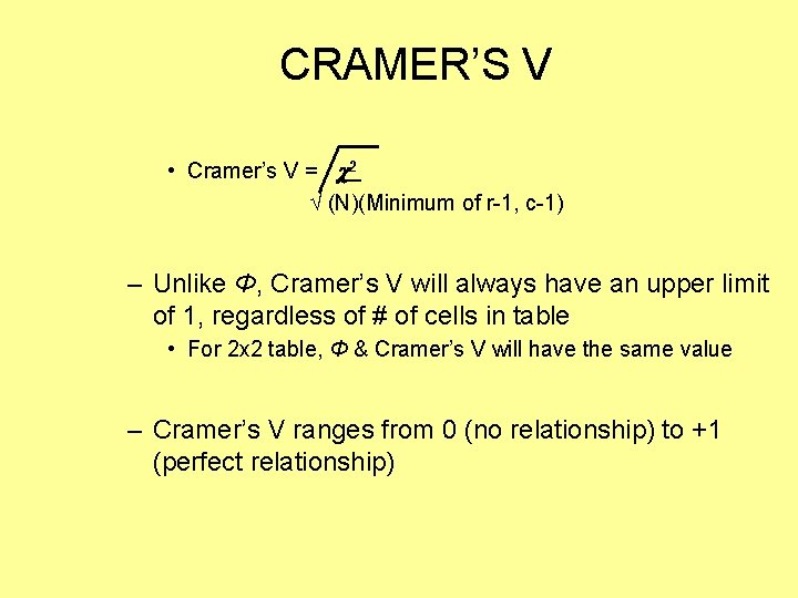
CRAMER’S V • Cramer’s V = 2 √ (N)(Minimum of r-1, c-1) – Unlike Φ, Cramer’s V will always have an upper limit of 1, regardless of # of cells in table • For 2 x 2 table, Φ & Cramer’s V will have the same value – Cramer’s V ranges from 0 (no relationship) to +1 (perfect relationship)

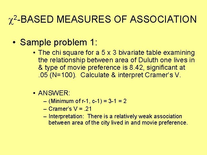
2 -BASED MEASURES OF ASSOCIATION • Sample problem 1: • The chi square for a 5 x 3 bivariate table examining the relationship between area of Duluth one lives in & type of movie preference is 8. 42, significant at. 05 (N=100). Calculate & interpret Cramer’s V. • ANSWER: – (Minimum of r-1, c-1) = 3 -1 = 2 – Cramer’s V =. 21 – Interpretation: There is a relatively weak association between area of the city lived in and movie preference.

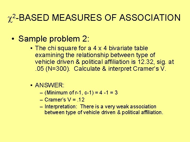
2 -BASED MEASURES OF ASSOCIATION • Sample problem 2: • The chi square for a 4 x 4 bivariate table examining the relationship between type of vehicle driven & political affiliation is 12. 32, sig. at. 05 (N=300). Calculate & interpret Cramer’s V. • ANSWER: – (Minimum of r-1, c-1) = 4 -1 = 3 – Cramer’s V =. 12 – Interpretation: There is a very weak association between type of vehicle driven & political affiliation.

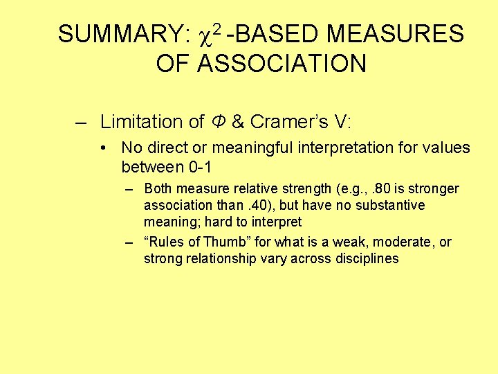
SUMMARY: 2 -BASED MEASURES OF ASSOCIATION – Limitation of Φ & Cramer’s V: • No direct or meaningful interpretation for values between 0 -1 – Both measure relative strength (e. g. , . 80 is stronger association than. 40), but have no substantive meaning; hard to interpret – “Rules of Thumb” for what is a weak, moderate, or strong relationship vary across disciplines

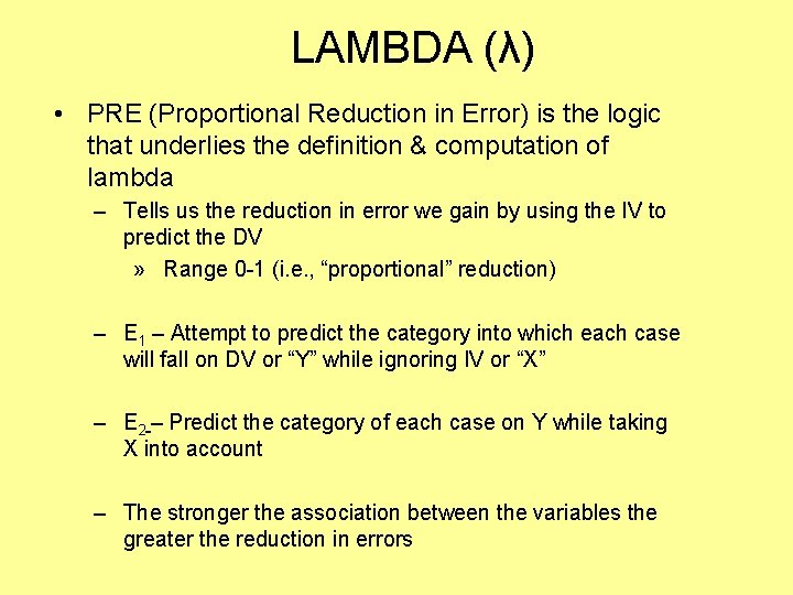
LAMBDA (λ) • PRE (Proportional Reduction in Error) is the logic that underlies the definition & computation of lambda – Tells us the reduction in error we gain by using the IV to predict the DV » Range 0 -1 (i. e. , “proportional” reduction) – E 1 – Attempt to predict the category into which each case will fall on DV or “Y” while ignoring IV or “X” – E 2 – Predict the category of each case on Y while taking X into account – The stronger the association between the variables the greater the reduction in errors

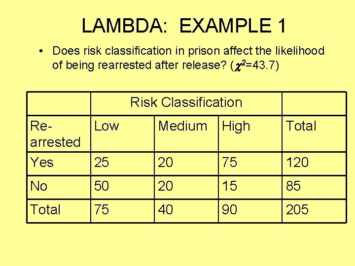
LAMBDA: EXAMPLE 1 • Does risk classification in prison affect the likelihood of being rearrested after release? ( 2=43. 7) Risk Classification Re. Low arrested Yes 25 Medium High Total 20 75 120 No 50 20 15 85 Total 75 40 90 205

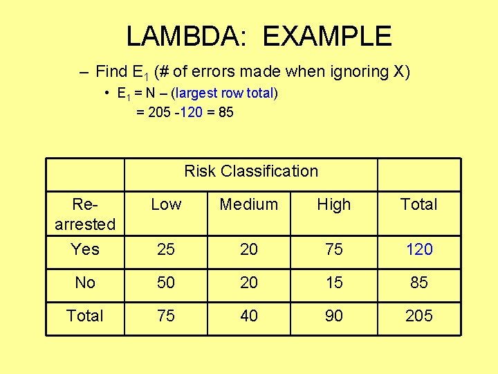
LAMBDA: EXAMPLE – Find E 1 (# of errors made when ignoring X) • E 1 = N – (largest row total) = 205 -120 = 85 Risk Classification Rearrested Low Medium High Total Yes 25 20 75 120 No 50 20 15 85 Total 75 40 90 205

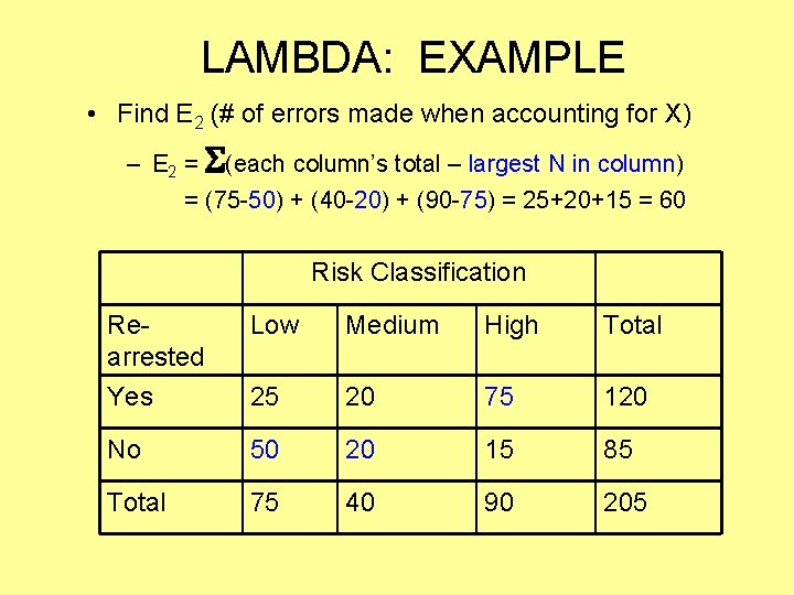
LAMBDA: EXAMPLE • Find E 2 (# of errors made when accounting for X) – E 2 = (each column’s total – largest N in column) = (75 -50) + (40 -20) + (90 -75) = 25+20+15 = 60 Risk Classification Rearrested Low Medium High Total Yes 25 20 75 120 No 50 20 15 85 Total 75 40 90 205

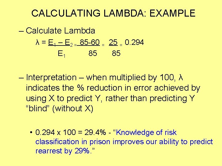
CALCULATING LAMBDA: EXAMPLE – Calculate Lambda λ = E 1 – E 2 = 85 -60 = 25 = 0. 294 E 1 85 85 – Interpretation – when multiplied by 100, λ indicates the % reduction in error achieved by using X to predict Y, rather than predicting Y “blind” (without X) • 0. 294 x 100 = 29. 4% - “Knowledge of risk classification in prison improves our ability to predict rearrest by 29%. ”

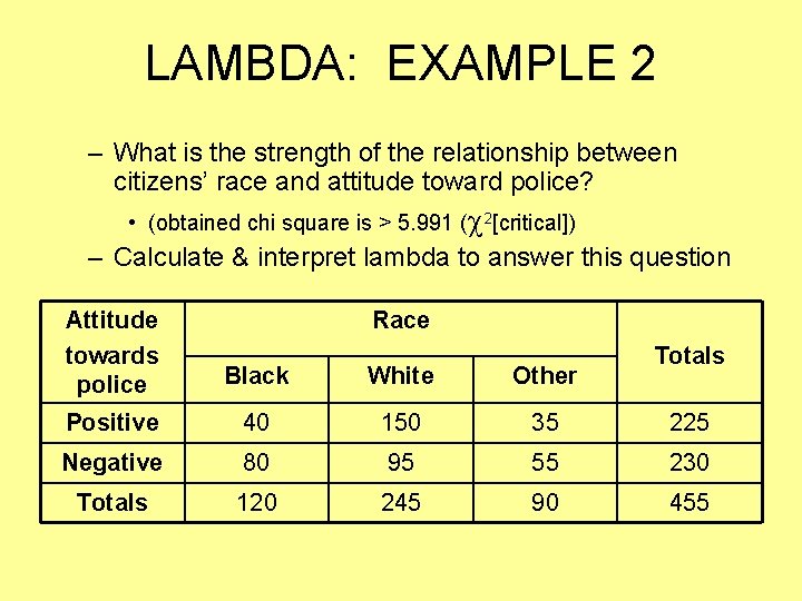
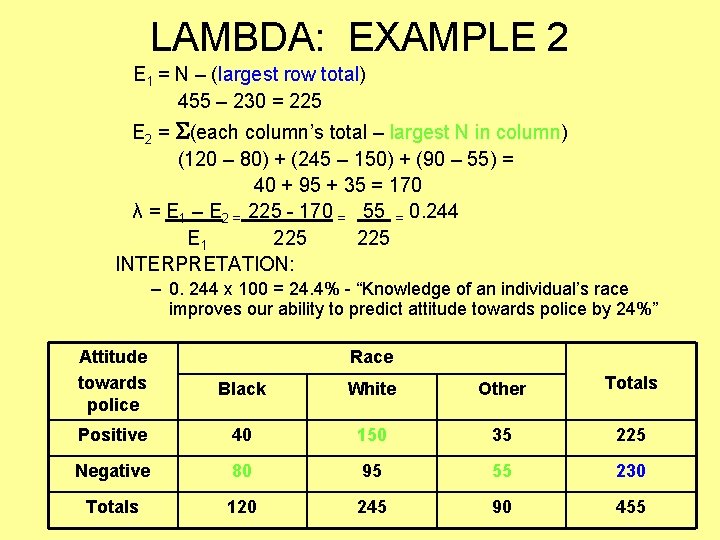
LAMBDA: EXAMPLE 2 – What is the strength of the relationship between citizens’ race and attitude toward police? • (obtained chi square is > 5. 991 ( 2[critical]) – Calculate & interpret lambda to answer this question Attitude towards police Race Black White Other Positive 40 150 35 225 Negative 80 95 55 230 Totals 120 245 90 455 Totals

LAMBDA: EXAMPLE 2 E 1 = N – (largest row total) 455 – 230 = 225 E 2 = (each column’s total – largest N in column) (120 – 80) + (245 – 150) + (90 – 55) = 40 + 95 + 35 = 170 λ = E 1 – E 2 = 225 - 170 = 55 = 0. 244 E 1 225 INTERPRETATION: – 0. 244 x 100 = 24. 4% - “Knowledge of an individual’s race improves our ability to predict attitude towards police by 24%” Attitude towards police Race Black White Other Totals Positive 40 150 35 225 Negative 80 95 55 230 Totals 120 245 90 455

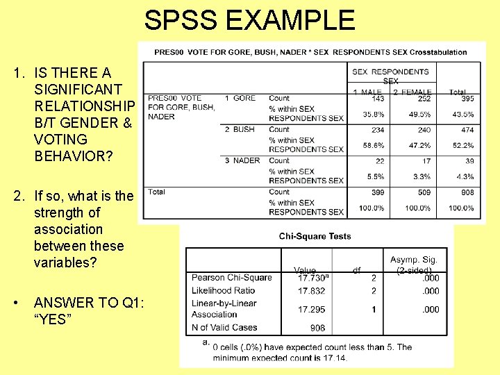
SPSS EXAMPLE 1. IS THERE A SIGNIFICANT RELATIONSHIP B/T GENDER & VOTING BEHAVIOR? 2. If so, what is the strength of association between these variables? • ANSWER TO Q 1: “YES”

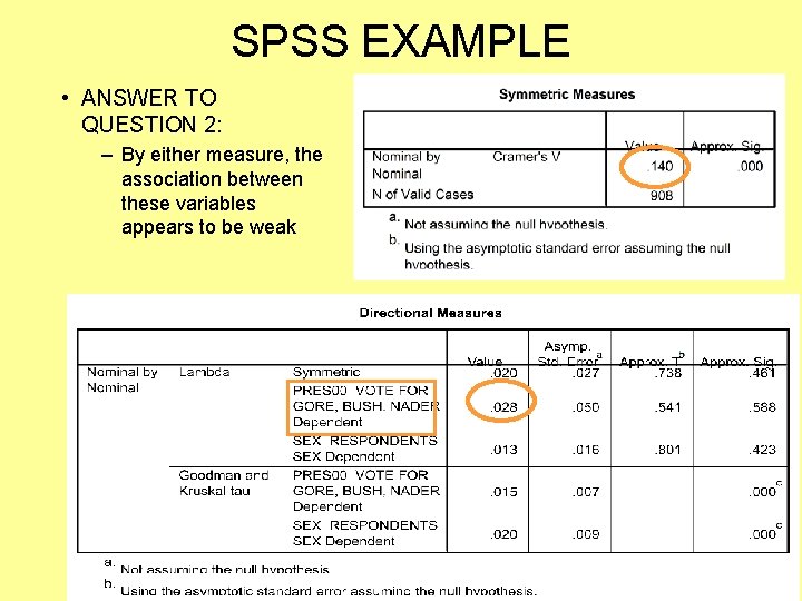
SPSS EXAMPLE • ANSWER TO QUESTION 2: – By either measure, the association between these variables appears to be weak

2 LIMITATIONS OF LAMBDA 1. Asymmetric • Value of the statistic will vary depending on which variable is taken as independent 2. Misleading when one of the row totals is much larger than the other(s) • For this reason, when row totals are extremely uneven, use a chi square-based measure instead

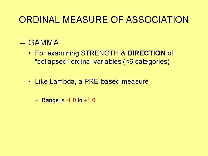
ORDINAL MEASURE OF ASSOCIATION – GAMMA • For examining STRENGTH & DIRECTION of “collapsed” ordinal variables (<6 categories) • Like Lambda, a PRE-based measure – Range is -1. 0 to +1. 0

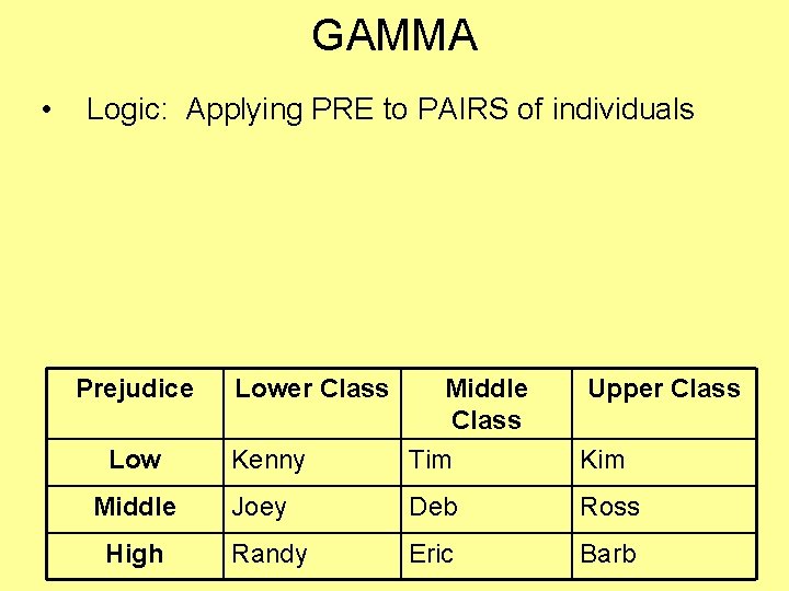
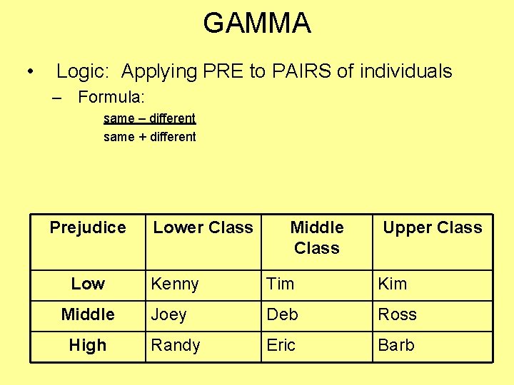
GAMMA • Logic: Applying PRE to PAIRS of individuals Prejudice Low Middle High Lower Class Middle Class Upper Class Kenny Tim Kim Joey Deb Ross Randy Eric Barb

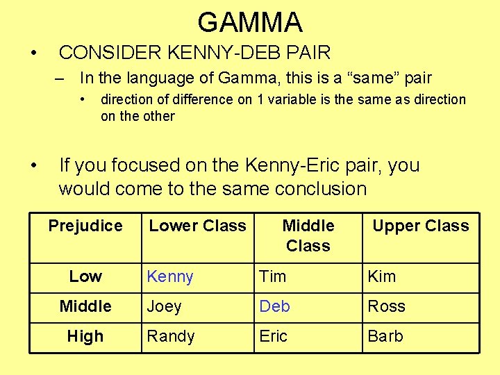
GAMMA • CONSIDER KENNY-DEB PAIR – In the language of Gamma, this is a “same” pair • • direction of difference on 1 variable is the same as direction on the other If you focused on the Kenny-Eric pair, you would come to the same conclusion Prejudice Low Middle High Lower Class Middle Class Upper Class Kenny Tim Kim Joey Deb Ross Randy Eric Barb

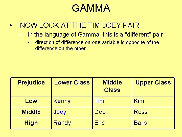
GAMMA • NOW LOOK AT THE TIM-JOEY PAIR – In the language of Gamma, this is a “different” pair • direction of difference on one variable is opposite of the difference on the other Prejudice Low Middle High Lower Class Middle Class Upper Class Kenny Tim Kim Joey Deb Ross Randy Eric Barb

GAMMA • Logic: Applying PRE to PAIRS of individuals – Formula: same – different same + different Prejudice Low Middle High Lower Class Middle Class Upper Class Kenny Tim Kim Joey Deb Ross Randy Eric Barb

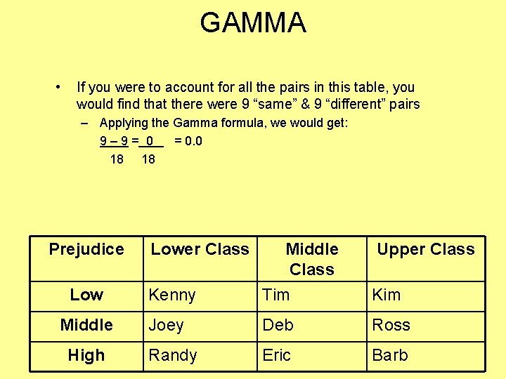
GAMMA • If you were to account for all the pairs in this table, you would find that there were 9 “same” & 9 “different” pairs – Applying the Gamma formula, we would get: 9– 9= 0 = 0. 0 18 18 Prejudice Low Middle High Lower Class Middle Class Upper Class Kenny Tim Kim Joey Deb Ross Randy Eric Barb

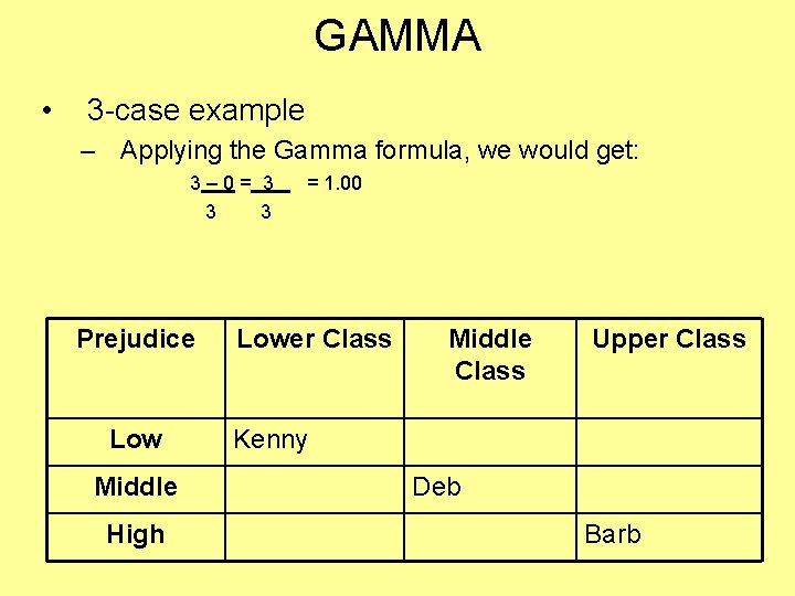
GAMMA • 3 -case example – Applying the Gamma formula, we would get: 3– 0= 3 3 3 Prejudice Low Middle High = 1. 00 Lower Class Middle Class Upper Class Kenny Deb Barb

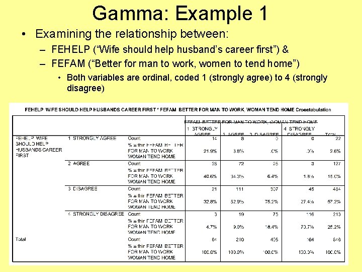
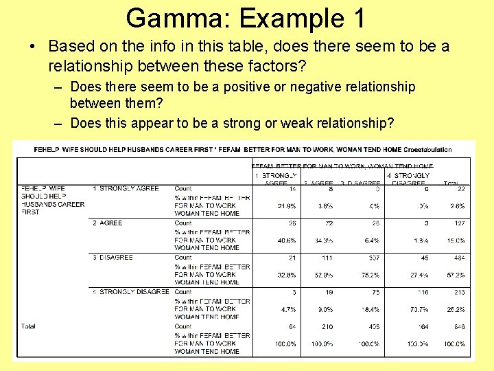
Gamma: Example 1 • Examining the relationship between: – FEHELP (“Wife should help husband’s career first”) & – FEFAM (“Better for man to work, women to tend home”) • Both variables are ordinal, coded 1 (strongly agree) to 4 (strongly disagree)

Gamma: Example 1 • Based on the info in this table, does there seem to be a relationship between these factors? – Does there seem to be a positive or negative relationship between them? – Does this appear to be a strong or weak relationship?

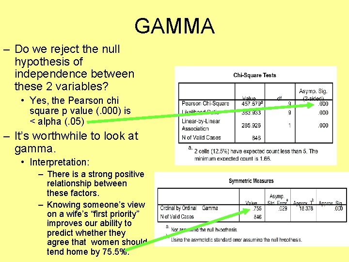
GAMMA – Do we reject the null hypothesis of independence between these 2 variables? • Yes, the Pearson chi square p value (. 000) is < alpha (. 05) – It’s worthwhile to look at gamma. • Interpretation: – There is a strong positive relationship between these factors. – Knowing someone’s view on a wife’s “first priority” improves our ability to predict whether they agree that women should tend home by 75. 5%.