1 mm Polarization Science with CARMA Chat Hull

1 mm Polarization Science with CARMA Chat Hull UC Berkeley, Radio Astronomy Laboratory Collaborators: Dick Plambeck, Greg Engargiola, & all the CARMA staff 12 October 2011 NSF Reverse Site Visit Washington, DC

1 mm Polarization: Science Goals • Magnetic-field morphology in Class 0 s – B-field vs. outflow direction – Using dust polarization and Goldreich-Kylafis effect • Polarization variability in Sgr A* – Probing time-variable accretion onto central BH • Collaborator interests – MHD turbulence

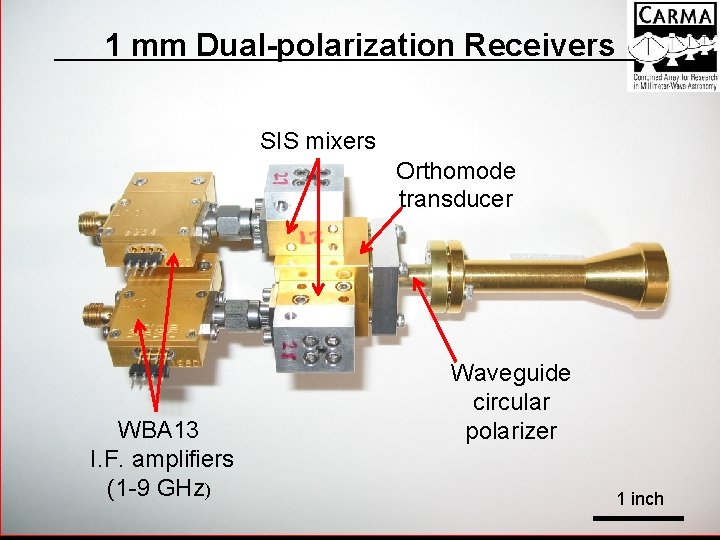
1 mm Dual-polarization Receivers SIS mixers Orthomode transducer WBA 13 I. F. amplifiers (1 -9 GHz) Waveguide circular polarizer 1 inch

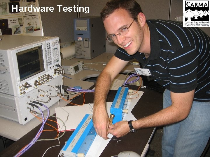
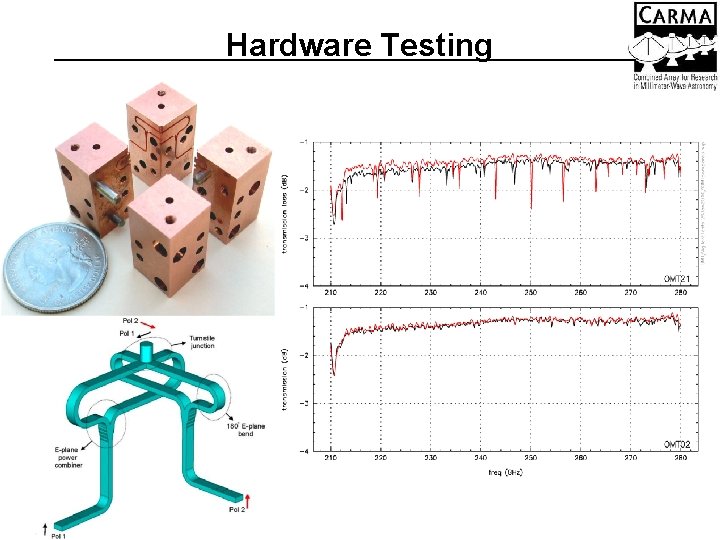
Hardware Testing

Hardware Testing

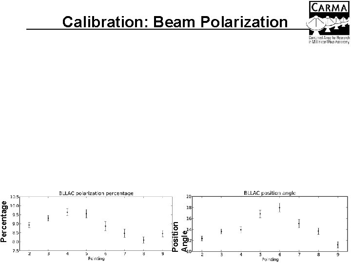
Position Angle Percentage Calibration: Beam Polarization

Calibration: XY Phase

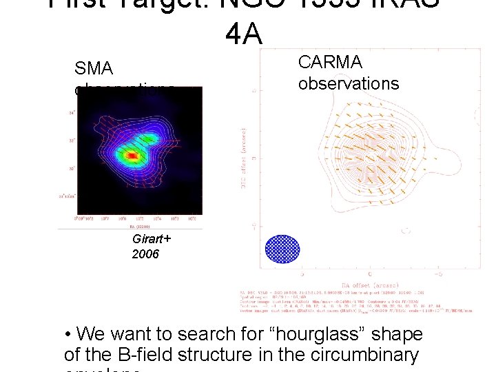
First Results: NGC 1333 -IRAS 4 A

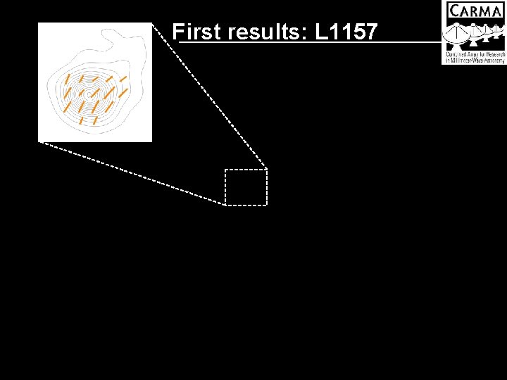
First results: L 1157

CARMA Combine Array for Research in Millimeter-wave Astronomy Consortium: Berkeley, Caltech, Illinois, Maryland, Chicago • Science goals – Molecular emission in galaxies – Galaxy clusters – Protoplanetary debris disks – Dust polarization in star-forming regions • Attributes – 6 � 10 -m, 9 � 6 -m, 8 � m telescopes – Observations at 1 mm, 3 mm, and 1 cm – Located in Cedar Flat, CA (near Bishop)

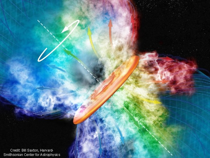
Credit: Bill Saxton, Harvard. Smithsonian Center for Astrophysics

First Target: NGC 1333 IRAS 4 A SMA observations CARMA observations Girart+ 2006 • We want to search for “hourglass” shape of the B-field structure in the circumbinary

Class 0 Dust Polarization Credit: NASA, ESA, STSc. I, J. Hester and P. Scowen (Arizona State

Why observe polarization? • B-fields play an important role in star formation • How important? • Are they strong (& ordered)? • Are they weak (& chaotic)? • B-fields polarization • Dust grains align their spin axes with B-fields • Dust emission is strong at 1 mm

How do we make it work? Grad student

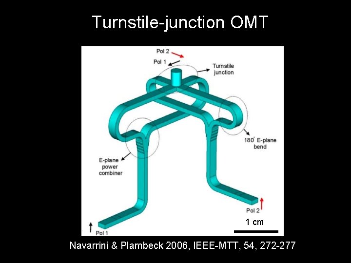
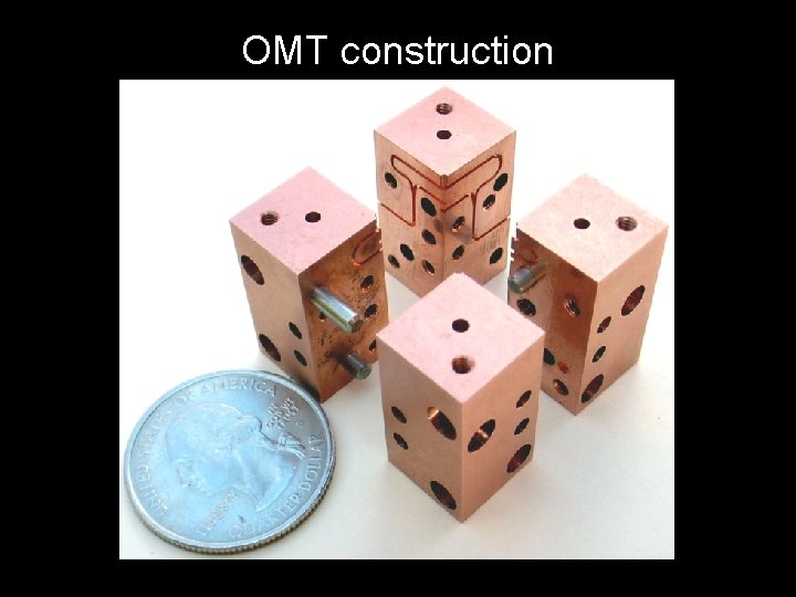
Turnstile-junction OMT 1 cm Navarrini & Plambeck 2006, IEEE-MTT, 54, 272 -277

OMT construction

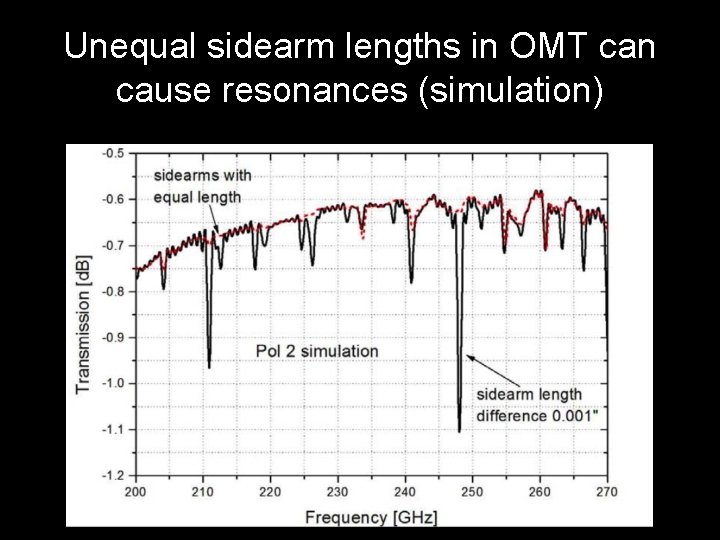
Unequal sidearm lengths in OMT can cause resonances (simulation)

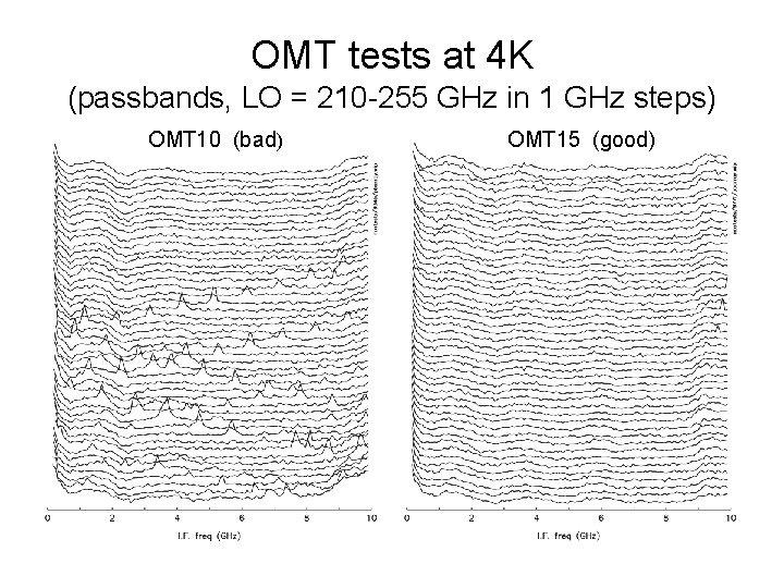
OMT tests at 4 K (passbands, LO = 210 -255 GHz in 1 GHz steps) OMT 10 (bad) OMT 15 (good)

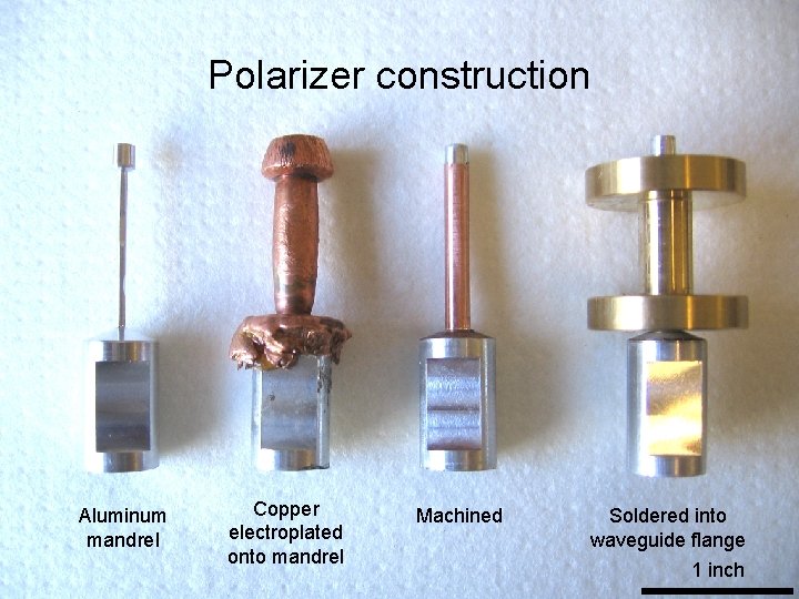
Polarizer construction Aluminum mandrel Copper electroplated onto mandrel Machined Soldered into waveguide flange 1 inch

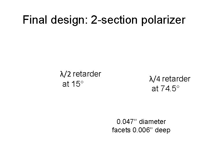
Final design: 2 -section polarizer λ/2 retarder at 15° λ/4 retarder at 74. 5° 0. 047’’ diameter facets 0. 006’’ deep

XY RL Receiv er Sk y

Fraction of linear radiation converted to RCP and LCP Sample polarizer test data (mandrel machining errors)

Polarization calibration • Two main steps to calibrate a polarimeter: – XY phase • The absolute phase offset between the RCP and LCP receivers of an antenna – Leakage terms • The fraction of LCP radiation detected in the RCP receiver, and vice versa

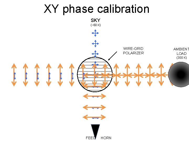
XY phase calibration • How do we find an antenna’s XY phase? – Observe a strongly polarized source with known position angle • These don’t exist at mm wavelengths • We create our own by observing broadband noise from the ambient load through a wire-grid polarizer!

XY phase calibration SKY (~60 K) WIRE-GRID POLARIZER AMBIENT LOAD (300 K) FEED HORN

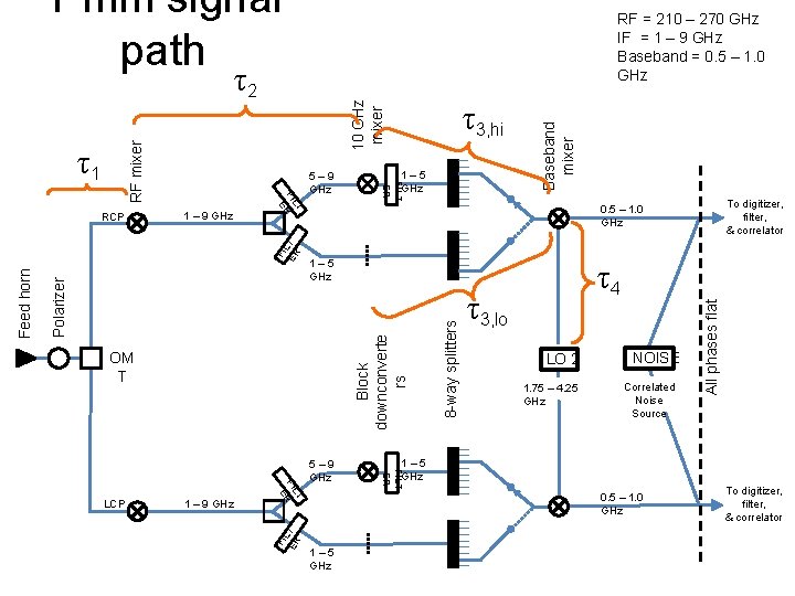
1 mm signal path 10 GHz mixer FI L ER T 5– 9 GHz τ4 τ3, lo LO 2 1. 75 – 4. 25 GHz NOISE Correlated Noise Source 1– 5 GHz 0. 5 – 1. 0 GHz 1– 5 GHz All phases flat Block downconverte rs Polarizer Feed horn 1– 5 GHz FILT ER LT FI R E 1 – 9 GHz To digitizer, filter, & correlator 0. 5 – 1. 0 GHz OM T LCP 1– 5 GHz 8 -way splitters 1 – 9 GHz FI L ER T RCP 5– 9 GHz τ3, hi FILT ER τ1 LT FI R E RF mixer τ2 Baseband mixer RF = 210 – 270 GHz IF = 1 – 9 GHz Baseband = 0. 5 – 1. 0 GHz To digitizer, filter, & correlator

Status/conclusions • Dual-polarization receivers are installed on all 15 6 - and 10 -m telescopes • Full-Stokes (LL, LR, RL, RR) system is working • Observed NGC 1333 -IRAS 4 A as a commissioning test • XY phase offset is well understood • Leakages need to be determined better • Will soon install new Berkeley-made polarizers