1 Lecture 11 Sorting Algorithms part II Quicksort

1 Lecture #11 • Sorting Algorithms, part II: – Quicksort – Mergesort • Introduction to Trees

2 But first… STL Challenge Give me a data structure that I can use to maintain a bunch of people’s names and for each person, allows me to easily get all of the streets they lived on. Assuming I have P total people and each person has lived on an average of E former streets… What is the Big-Oh cost of: A. Finding the names of all people who have lived on “Levering street”? B. Determining if “Bill” ever lived on “Westwood blvd”? C. Printing out every name along with each person’s street addresses, in alphabetical order. D. Printing out all of the streets that “Tala” has lived on.

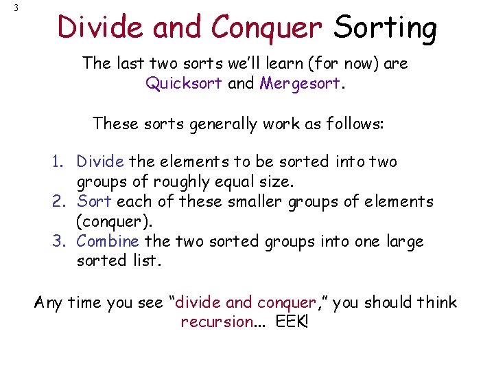
3 Divide and Conquer Sorting The last two sorts we’ll learn (for now) are Quicksort and Mergesort. These sorts generally work as follows: 1. Divide the elements to be sorted into two groups of roughly equal size. 2. Sort each of these smaller groups of elements (conquer). 3. Combine the two sorted groups into one large sorted list. Any time you see “divide and conquer, ” you should think recursion. . . EEK!

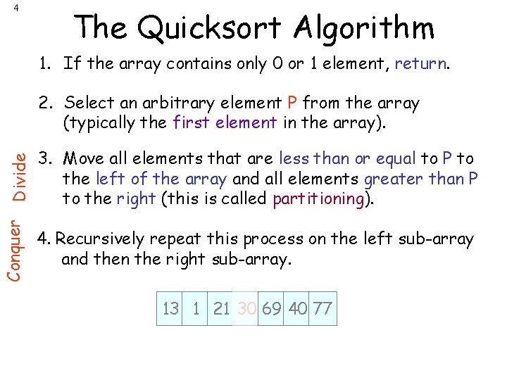
4 The Quicksort Algorithm 1. If the array contains only 0 or 1 element, return. Conquer Divide 2. Select an arbitrary element P from the array (typically the first element in the array). 3. Move all elements that are less than or equal to P to the left of the array and all elements greater than P to the right (this is called partitioning). 4. Recursively repeat this process on the left sub-array and then the right sub-array. 30 13 69 40 77 21 13 1 77 21 30

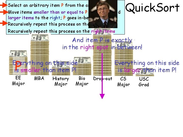
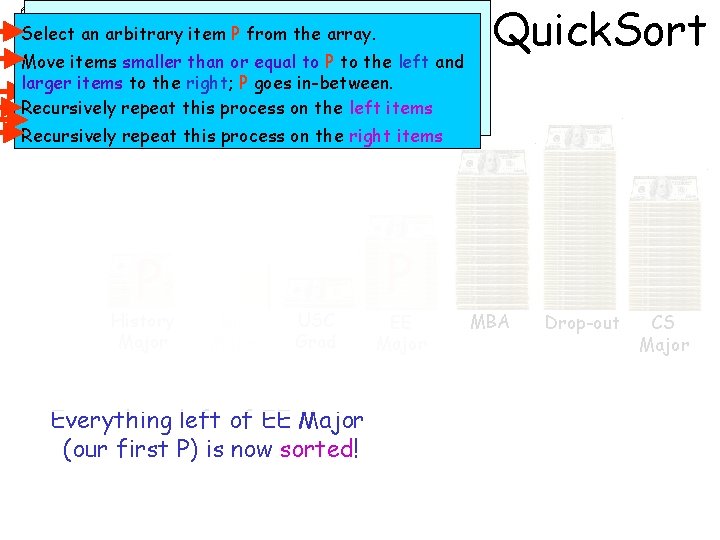
5 Select an arbitrary item P from the array. Move items smaller than or equal to P to the left and larger items to the right; P goes in-between. Recursively repeat this process on the left items Quick. Sort Recursively repeat this process on the right items And item P is exactly in the right spot in between! P Everything on this side is smaller than item P! EE Major MBA History Major Bio Major Everything on this side is larger than item P! Drop-out CS Major USC Grad

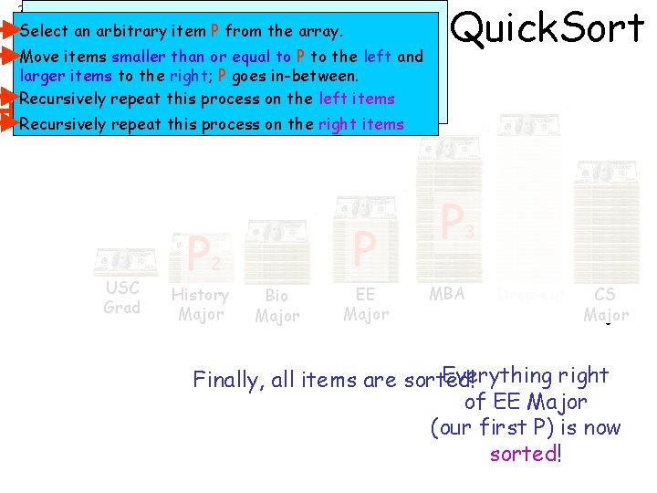
6 Select an arbitrary item P from the array. Move items smaller than or equal to P to the left and Move items smaller or. Pequal P to the left and larger items to thethan right; goes to in-between. larger items to the right; P goes in-between. Recursively repeat this process on the left items Recursively repeat this process on the right items P P 2 History Major Quick. Sort Bio Major USC Grad Everything left of EE Major (our first P) is now sorted! EE Major MBA Drop-out CS Major

7 Select an arbitrary item P from the array. Move items smaller than or equal to P to the left and Move items smaller or. Pequal P to the left and larger items to thethan right; goes to in-between. larger items to the right; P goes in-between. Recursively repeat this process on the left items Recursively repeat this process on the right items USC Grad P P 2 History Major Bio Major EE Major Quick. Sort P 3 MBA Drop-out CS Major Everything right Finally, all items are sorted! of EE Major (our first P) is now sorted!

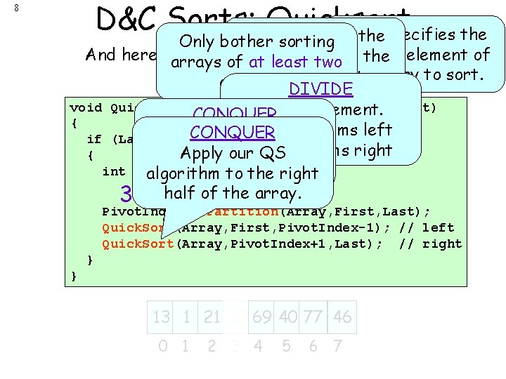
D&C Sorts: Last. Quicksort First specifies the 8 Only bother sorting starting element of And here’s arrays an actual Quicksort C++ function: element of the oflast at least two the array to sort. elements! 0 7 DIVIDE void Quick. Sort(int Array[], int First, int Last) Pick an element. CONQUER { Move <= items left CONQUER Apply our if (Last – First >= 1 QS ) > items right Apply our QS left { algorithm to. Move the int Pivot. Index; algorithm to the right half of the array. 3 half of the array. Pivot. Index = Partition(Array, First, Last); Quick. Sort(Array, First, Pivot. Index-1); // left Quick. Sort(Array, Pivot. Index+1, Last); // right } } 30 13 1 77 21 30 13 69 40 77 21 46 0 1 2 3 4 5 6 7

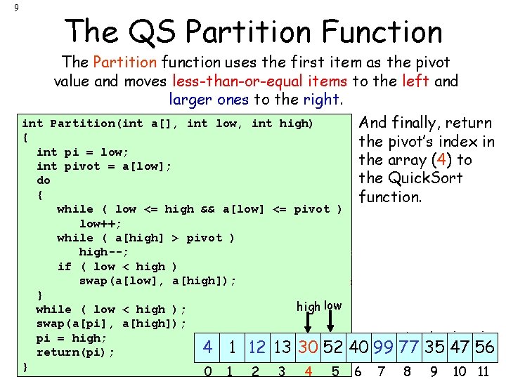
9 The QS Partition Function The Partition function uses the first item as the pivot value and moves less-than-or-equal items to the left and larger ones to the right. int Partition(int a[], int low, int high) And finally, return { the pivot’s index in int pi = low; the to ourarray pivot (4) value int pivot = a[low]; } – Select the first item as the Quick. Sort do { function. value Find first next value }}- while ( low <= high && a[low] <= pivot ) low++; >> than the pivot. Find first next value while ( a[high] > pivot ) high--; <= <= than the pivot. if ( low < high ) high Swap pivot to proper swap(a[low], a[high]); } – Swap the larger with the smaller }- } while ( low < high ); swap(a[pi], a[high]); pi = high; return(pi); } position in array low low highhighhigh } – done }– 30 99 4 77 12 35 47 56 4 1 77 12 13 30 4 52 40 99 0 1 2 3 4 5 6 7 8 9 10 11

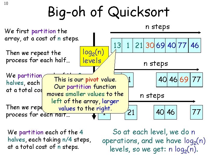
10 Big-oh of Quicksort n steps We first partition the array, at a cost of n steps. Then we repeat the process for each half… log 2(n) levels 30 13 69 40 77 21 46 13 1 77 21 30 We partition each of the 2 This is our pivot value. 13 1 21 1 13 halves, each taking n/2 steps, Our partition function at a total cost of n steps. moves smaller values to the left of the array, larger Then we repeat thevalues to the right. 1 21 process for each half… We partition each of the 4 halves, each taking n/4 steps, at a total cost of n steps 69 40 40 46 77 69 46 77 n steps 40 46 77 So at each level, we do n operations, and we have log 2(n) levels, so we get: n log 2(n).

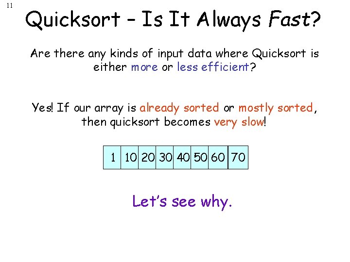
11 Quicksort – Is It Always Fast? Are there any kinds of input data where Quicksort is either more or less efficient? Yes! If our array is already sorted or mostly sorted, then quicksort becomes very slow! 1 10 20 30 40 50 60 70 Let’s see why.

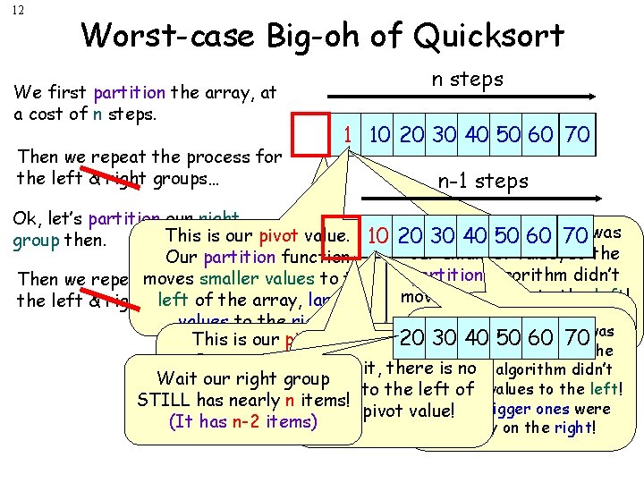
12 Worst-case Big-oh of Quicksort We first partition the array, at a cost of n steps. Then we repeat the process for the left & right groups… n steps 1 10 20 30 40 50 60 70 n-1 steps Ok, let’s partition our right Wait! pivot This is our pivot value. 10 20 30 Our 40 50 60 value 70 was group then. our smallest value, so the Our partition But function wait, there is no partition algorithm didn’t smallerfor values Then we repeatmoves the process grouptotothe left of move any values to the left! left of the array, the larger the left & right groups… pivot value! All the bigger onesright were Wait our values to the right. Wait! Our pivot value was already on 50 the 60 right This is our pivot value. 20 30 40 70 side! group STILL has our smallest value, so the Our partition But function n items! wait, therepartition is no nearly algorithm didn’t Wait our right group moves smaller values (It has n-1 items) any values to the left! grouptotothe move left of STILLleft hasof nearly n items! the array, the larger All the bigger ones were pivot value! (It has n-2 to items) values the right. already on the right!

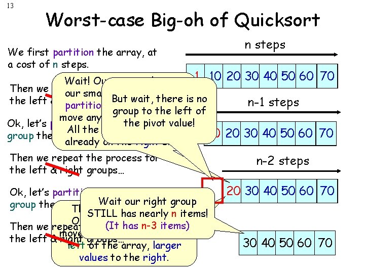
13 Worst-case Big-oh of Quicksort We first partition the array, at a cost of n steps. Wait! Our pivot value was 1 10 Then we repeat the process for our smallest value, so the But wait, there is no the left & right groups… partition algorithm didn’t group to the left of move any values to the left! the pivot value! Ok, let’s partition our right All the bigger ones were 10 group then. already on the right side! Then we repeat the process for the left & right groups… Ok, let’s partition our right group then. This is. Wait ourhas pivot value. STILL nearly n items! Our partition hasfunction n-3 Then we repeat the (It process foritems) moves smaller values to the left & right groups… left of the array, larger values to the right. n steps 20 30 40 50 60 70 n-1 steps 20 30 40 50 60 70 n-2 steps 20 30 40 50 60 70

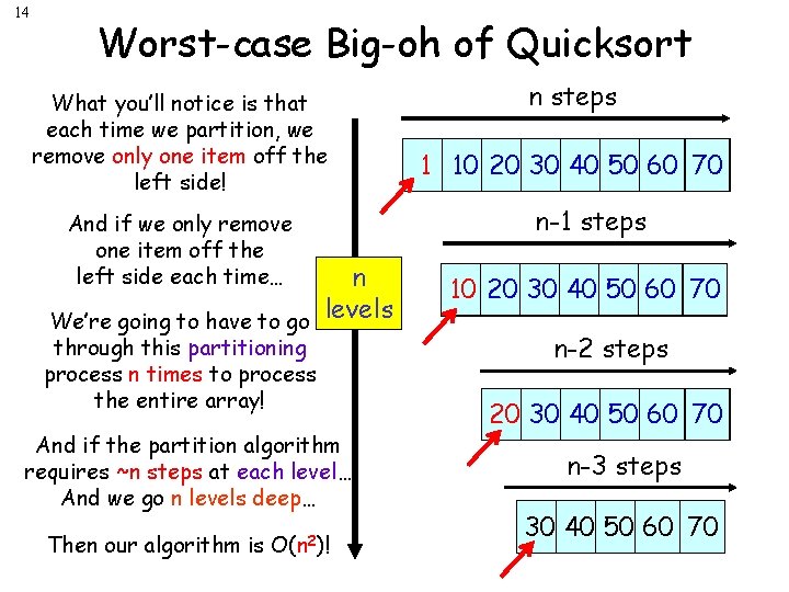
14 Worst-case Big-oh of Quicksort What you’ll notice is that each time we partition, we remove only one item off the left side! And if we only remove one item off the left side each time… n We’re going to have to go levels through this partitioning process n times to process the entire array! And if the partition algorithm requires ~n steps at each level… And we go n levels deep… Then our algorithm is O(n 2)! n steps 1 10 20 30 40 50 60 70 n-1 steps 10 20 30 40 50 60 70 n-2 steps 20 30 40 50 60 70 n-3 steps 30 40 50 60 70

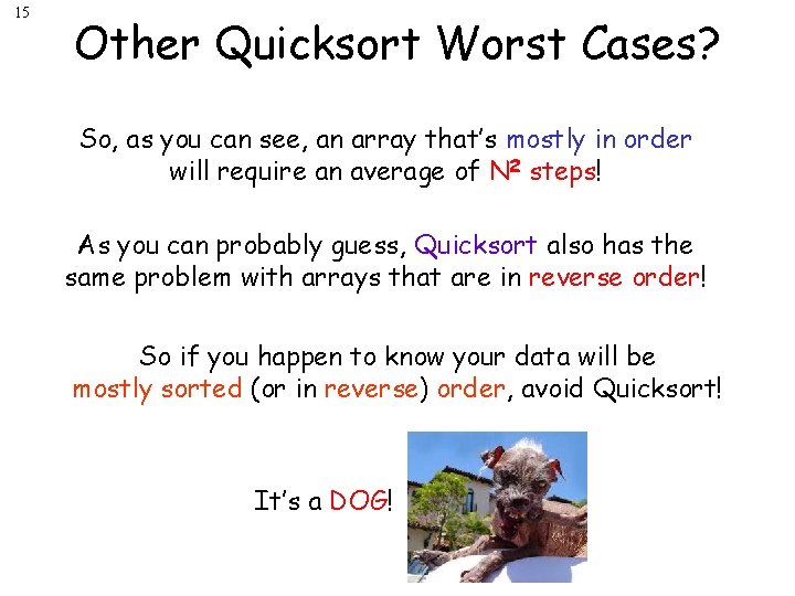
15 Other Quicksort Worst Cases? So, as you can see, an array that’s mostly in order will require an average of N 2 steps! As you can probably guess, Quicksort also has the same problem with arrays that are in reverse order! So if you happen to know your data will be mostly sorted (or in reverse) order, avoid Quicksort! It’s a DOG!

16 Quick. Sort Questions Can Quick. Sort be applied easily to sort items within a linked list? Is Quick. Sort a “stable” sort? Does Quick. Sort use a fixed amount of RAM, or can it vary? Can Quick. Sort be parallelized across multiple cores? When might you use Quick. Sort?

17 Mergesort The Mergesort is another extremely efficient sort – yet it’s pretty easy to understand. But before we learn the Mergesort, we need to learn another algorithm called “merge”.

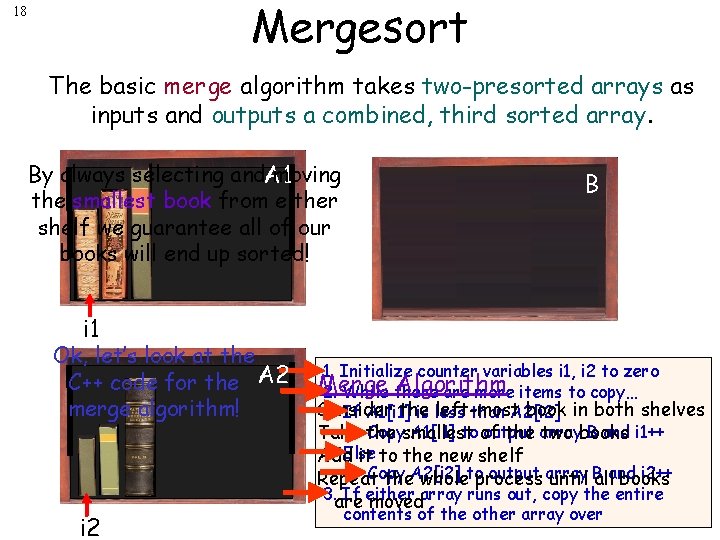
Mergesort 18 The basic merge algorithm takes two-presorted arrays as inputs and outputs a combined, third sorted array. By always selecting and. A 1 moving the smallest book from either shelf we guarantee all of our books will end up sorted! B i 1 Ok, let’s look at the C++ code for the A 2 merge algorithm! i 2 1. Initialize counter variables i 1, i 2 to zero Merge Algorithm 2. While there are more items to copy… Consider the left-most book in both shelves If A 1[i 1] is less than A 2[i 2] Copysmallest A 1[i 1] to of output B and i 1++ Take the array two books Else Add it to the new shelf Copy output array i 2++ Repeat the. A 2[i 2] wholetoprocess until B alland books 3. are If either movedarray runs out, copy the entire contents of the other array over

19 Merge Algorithm in C++ void merge(int data[], int n 1, int n 2) { int i=0, j=0, k=0; int *temp = new int[n 1+n 2]; int *sechalf = data + n 1; Here’s the C++ version of our merge function! while (i < n 1 || j < n 2) { if (i == n 1) temp[k++] = sechalf[j++]; else if (j == n 2) temp[k++] = data[i++]; else if (data[i] < sechalf[j]) temp[k++] = data[i++]; else temp[k++] = sechalf[j++]; } for (i=0; i<n 1+n 2; i++) data 1 13 data[i] = temp[i]; 5 delete [] temp; you pass in an array called data and two sizes: n 1 and n 2 } Instead of passing in A 1, A 2 and B… Notice how this function uses new/delete to allocate a temporary array for merging. data holds the merged contents at the end. 213`040 5 40 13 19 21 69 77 5 30 13 19 69 30 40 20 19 20 21 13 13 n 1=6 n 2=4

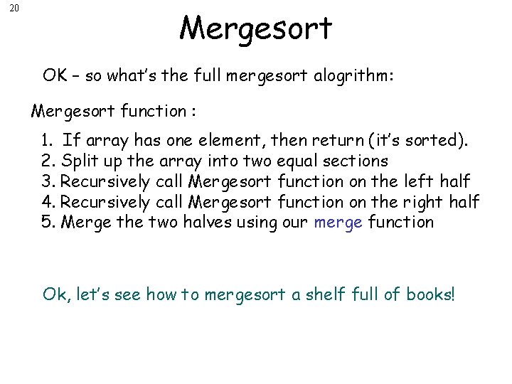
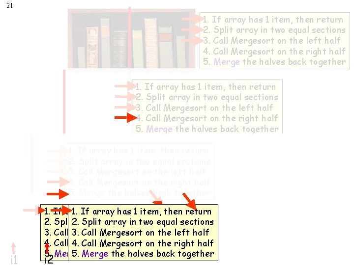
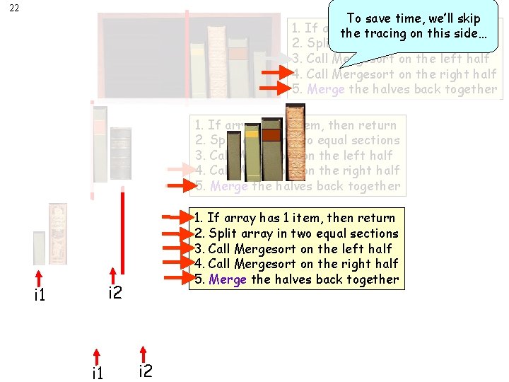
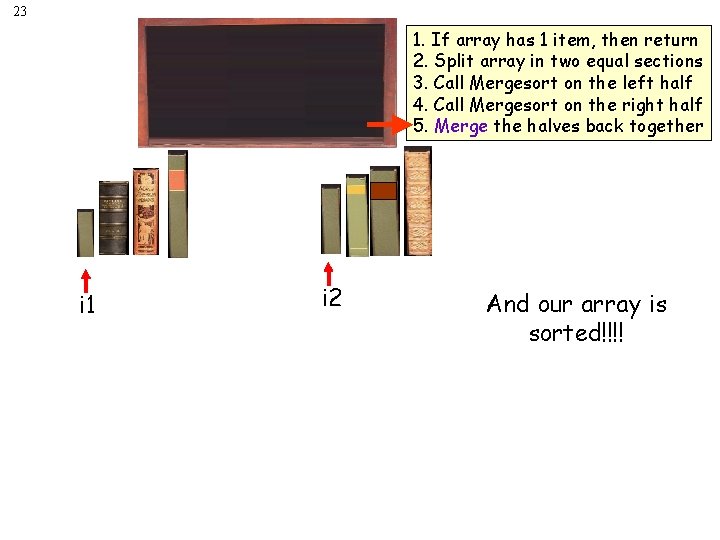
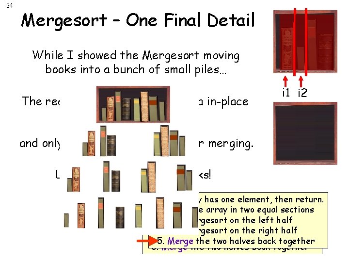
20 Mergesort OK – so what’s the full mergesort alogrithm: Mergesort function : 1. If array has one element, then return (it’s sorted). 2. Split up the array into two equal sections 3. Recursively call Mergesort function on the left half 4. Recursively call Mergesort function on the right half 5. Merge the two halves using our merge function Ok, let’s see how to mergesort a shelf full of books!

21 1. If array has 1 item, then return 2. Split array in two equal sections 3. Call Mergesort on the left half 4. Call Mergesort on the right half 5. Merge the halves back together i 1 1. If array 1 item, 1. Ifhas array has 1 then item, return then return 2. Split 2. array two equal Splitinarray in twosections equal sections 3. Call 3. Mergesort on the on left half Call Mergesort the left half 4. Call 4. Mergesort on the on right Call Mergesort thehalf right half 5. Merge the halves back together i 2

22 To save time, we’ll skip 1. If array 1 item, return thehas tracing on then this side… 2. Split array in two equal sections 3. Call Mergesort on the left half 4. Call Mergesort on the right half 5. Merge the halves back together 1. If array has 1 item, then return 2. Split array in two equal sections 3. Call Mergesort on the left half 4. Call Mergesort on the right half 5. Merge the halves back together i 2 i 1 i 2

23 1. If array has 1 item, then return 2. Split array in two equal sections 3. Call Mergesort on the left half 4. Call Mergesort on the right half 5. Merge the halves back together i 1 i 2 And our array is sorted!!!!

24 Mergesort – One Final Detail While I showed the Mergesort moving books into a bunch of small piles… The real algorithm sorts the data in-place in the array… i 1 i 2 and only uses a separate array for merging. Let’s see how it really works! 1. If array has one element, then return. 2. Split the array in two equal sections 3. Call Mergesort on the left half 4. Call Mergesort on the right half 5. Merge the two halves back together

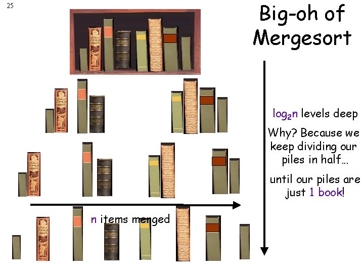
Big-oh of Mergesort 25 log 2 n levels deep Why? Because we keep dividing our piles in half… until our piles are just 1 book! n items merged

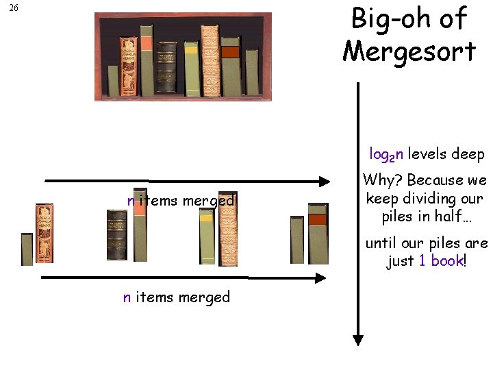
Big-oh of Mergesort 26 log 2 n levels deep n items merged Why? Because we keep dividing our piles in half… until our piles are just 1 book! n items merged

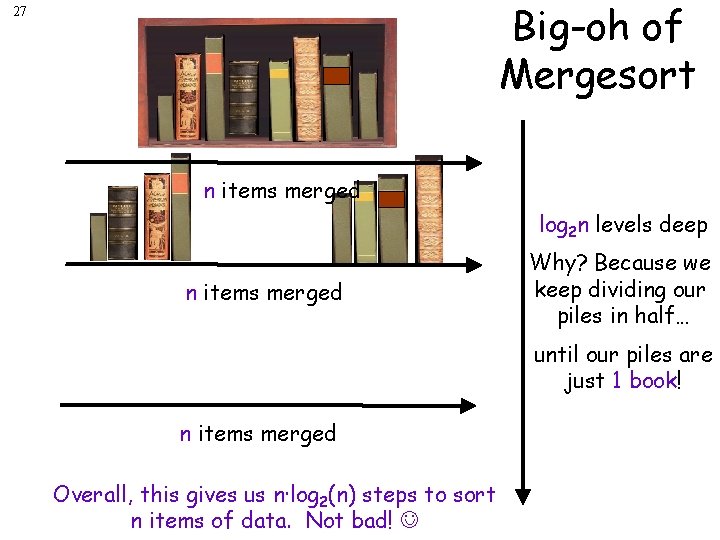
Big-oh of Mergesort 27 n items merged log 2 n levels deep n items merged Why? Because we keep dividing our piles in half… until our piles are just 1 book! n items merged Overall, this gives us n·log 2(n) steps to sort n items of data. Not bad!

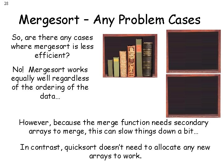
28 Mergesort – Any Problem Cases So, are there any cases where mergesort is less efficient? No! Mergesort works equally well regardless of the ordering of the data… However, because the merge function needs secondary arrays to merge, this can slow things down a bit… In contrast, quicksort doesn’t need to allocate any new arrays to work.

29 Merge. Sort Questions Can Merge. Sort be applied easily to sort items within a linked list? Is Merge. Sort a “stable” sort? Are there any special uses for Merge. Sort that other sorts can’t handle? Can Merge. Sort be parallelized across multiple cores?

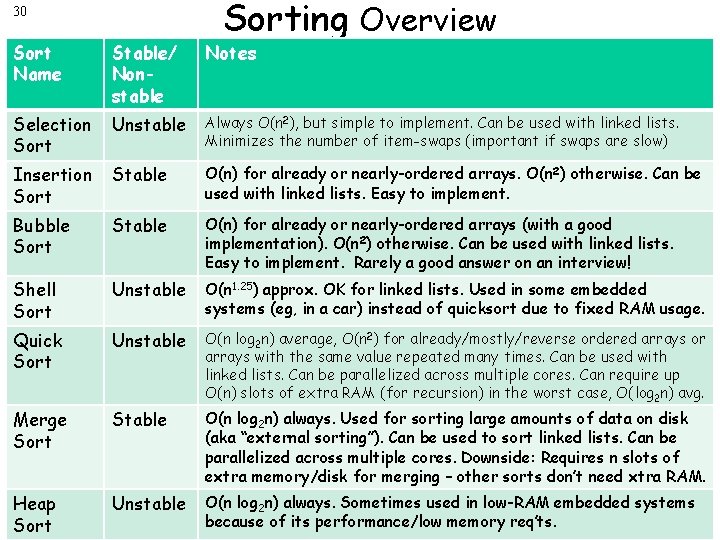
30 Sorting Overview Sort Name Stable/ Nonstable Notes Selection Sort Unstable Always O(n 2), but simple to implement. Can be used with linked lists. Minimizes the number of item-swaps (important if swaps are slow) Insertion Sort Stable O(n) for already or nearly-ordered arrays. O(n 2) otherwise. Can be used with linked lists. Easy to implement. Bubble Sort Stable O(n) for already or nearly-ordered arrays (with a good implementation). O(n 2) otherwise. Can be used with linked lists. Easy to implement. Rarely a good answer on an interview! Shell Sort Unstable O(n 1. 25) approx. OK for linked lists. Used in some embedded systems (eg, in a car) instead of quicksort due to fixed RAM usage. Quick Sort Unstable O(n log 2 n) average, O(n 2) for already/mostly/reverse ordered arrays or arrays with the same value repeated many times. Can be used with linked lists. Can be parallelized across multiple cores. Can require up O(n) slots of extra RAM (for recursion) in the worst case, O(log 2 n) avg. Merge Sort Stable O(n log 2 n) always. Used for sorting large amounts of data on disk (aka “external sorting”). Can be used to sort linked lists. Can be parallelized across multiple cores. Downside: Requires n slots of extra memory/disk for merging – other sorts don’t need xtra RAM. Heap Sort Unstable O(n log 2 n) always. Sometimes used in low-RAM embedded systems because of its performance/low memory req’ts.

31 Challenge Problems 1. Give an algorithm to efficiently determine which element occurs the largest number of times in the array. 2. What’s the best algorithm to sort 1, 000 random numbers that are all between 1 and 5?

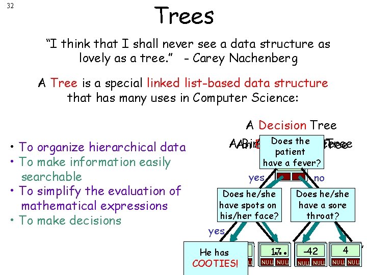
32 Trees “I think that I shall never see a data structure as lovely as a tree. ” - Carey Nachenberg A Tree is a special linked list-based data structure that has many uses in Computer Science: A Decision Tree • To organize hierarchical data • To make information easily searchable • To simplify the evaluation of mathematical expressions • To make decisions Does the. Tree AAn Binary A Family Search Tree Expression Tree patient have a+fever? “marty” “carey” yes no Does he/she have “harry” spots “leon” * on his/her face? yes … Does he/she have a sore “andrea” “rich” throat? + “nancy” “jacob” “simon” “zai” “sheila” “alan” 4 32 -42 “milton” 17 “martha” He has NULL NULL NULL NULL COOTIES!

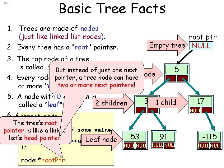
Basic Tree Facts 33 1. Trees are made of nodes (just like linked list nodes). root ptr Empty tree NULL 2. Every tree has a "root" pointer. 3. The top node of a tree is called its But "root" node. instead of just one next Root node pointer, a tree 4. Every node may have zeronode can have two or nodes. more next pointers! or more “children” 5. A node with 0 children is 2 children called a “leaf” node. 5 -33 1 child NULL 6. A struct tree with no nodes is node { tree’s The called anroot “empty tree. ” int pointer is likevalue; a linked // some value list’s head Leaf nodepointer! *left, *right; 0 children }; node *root. Ptr; 17 53 91 -115 NULL NULL

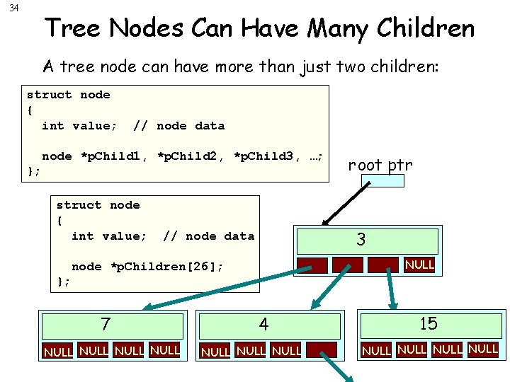
34 Tree Nodes Can Have Many Children A tree node can have more than just two children: struct node { int value; // node data node *p. Child 1, *p. Child 2, *p. Child 3, …; }; struct node { int value; root ptr 3 // node data NULL node *p. Children[26]; }; 7 NULL 4 NULL 15 NULL

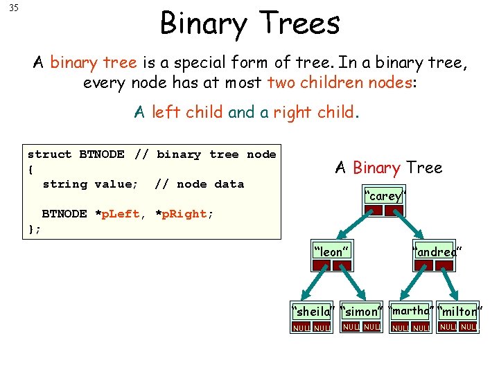
Binary Trees 35 A binary tree is a special form of tree. In a binary tree, every node has at most two children nodes: A left child and a right child. struct BTNODE // binary tree node { string value; // node data A Binary Tree “carey” BTNODE *p. Left, *p. Right; }; “leon” “andrea” “sheila” “simon” “martha” “milton” NULL NULL

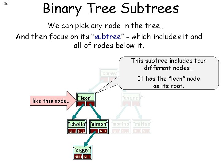
36 Binary Tree Subtrees We can pick any node in the tree… And then focus on its “subtree” - which includes it and all of nodes below it. This subtree includes four different nodes… “carey” like this node… It has the “leon” node as its root. “andrea” “leon” “sheila” “simon” “martha” “milton” NULL “ziggy” NULL NULL

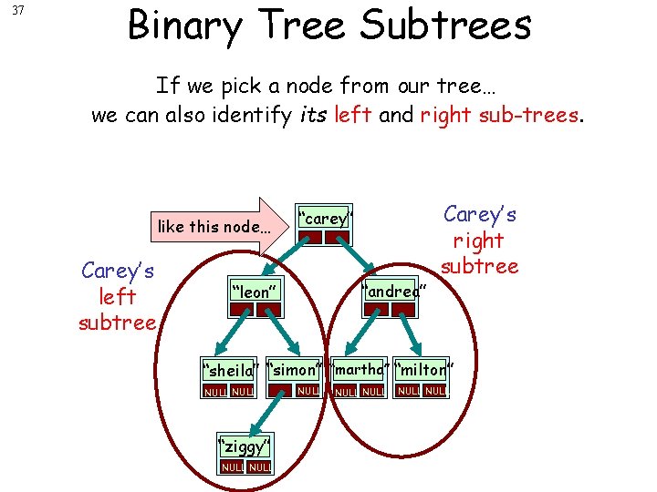
37 Binary Tree Subtrees If we pick a node from our tree… we can also identify its left and right sub-trees. like this node… Carey’s left subtree “carey” “andrea” “leon” Carey’s right subtree “sheila” “simon” “martha” “milton” NULL “ziggy” NULL NULL

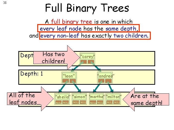
Full Binary Trees 38 A full binary tree is one in which every leaf node has the same depth, and every non-leaf has exactly two children. Depth: 0 Has two children! Depth: 1 All of the 2 Depth: leaf nodes… “carey” “leon” “andrea” “sheila” “simon” “martha” “milton” NULL NULL Are at the same depth!

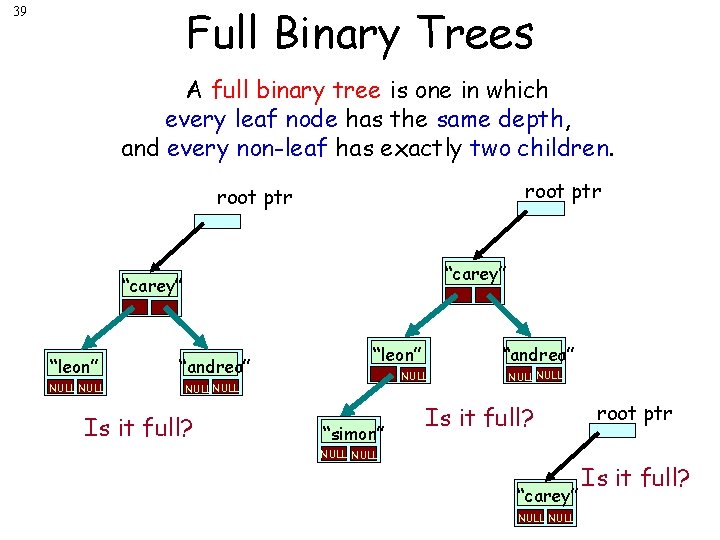
Full Binary Trees 39 A full binary tree is one in which every leaf node has the same depth, and every non-leaf has exactly two children. root ptr “carey” “leon” “andrea” NULL Is it full? “andrea” “leon” NULL “simon” NULL Is it full? NULL “carey” NULL root ptr Is it full?

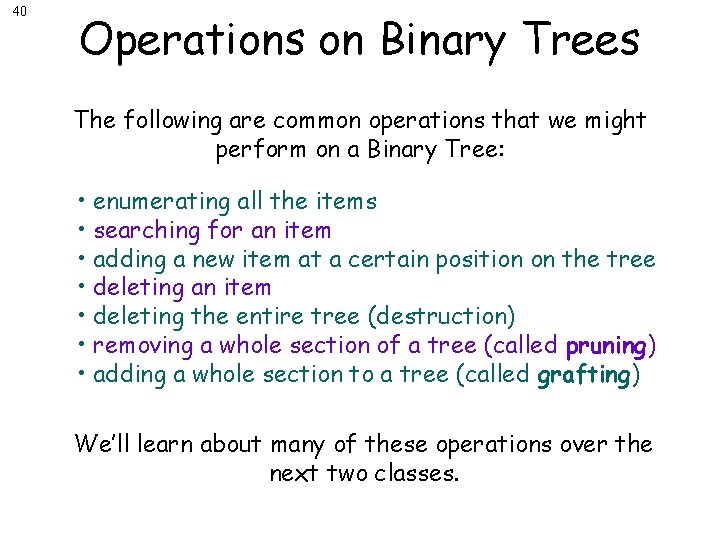
40 Operations on Binary Trees The following are common operations that we might perform on a Binary Tree: • enumerating all the items • searching for an item • adding a new item at a certain position on the tree • deleting an item • deleting the entire tree (destruction) • removing a whole section of a tree (called pruning) • adding a whole section to a tree (called grafting) We’ll learn about many of these operations over the next two classes.

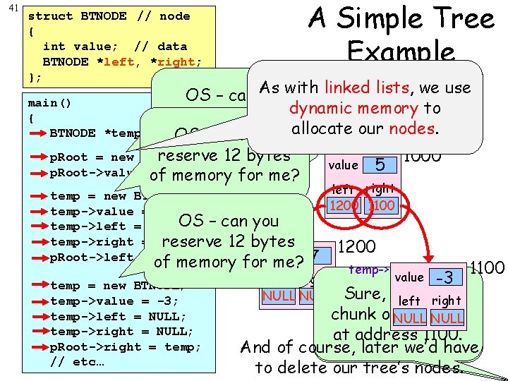
41 A Simple Tree Example struct BTNODE // node { int value; // data BTNODE *left, *right; }; temp 1200 1100 lists, we use As with linked OS – can you main() dynamic memory to p. Root 1000 reserve 12 bytes { allocate our nodes. BTNODE *temp, *p. Root; – can you of. OS memory for me? reserve 12 bytes p. Root = new BTNODE; 1000 value 5 p. Root->value of = 5; memory for me? temp = new BTNODE; temp->value = 7; OS – can you temp->left = NULL; temp->right = NULL; reservetemp-> 12 bytes value p. Root->left = temp; of memory for me? 7 temp = new BTNODE; temp->value = -3; temp->left = NULL; temp->right = NULL; p. Root->right = temp; // etc… left right 1200 1100 1200 temp-> 1100 -3 Sure, here’s a left right chunk of. NULL memory NULL at address 1200. 1100. 1000. And of course, later we’d have to delete our tree’s nodes. left right NULL value

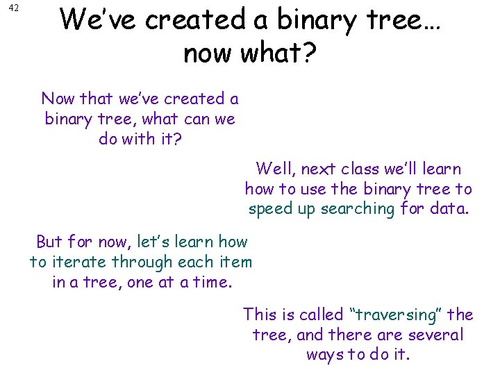
42 We’ve created a binary tree… now what? Now that we’ve created a binary tree, what can we do with it? Well, next class we’ll learn how to use the binary tree to speed up searching for data. But for now, let’s learn how to iterate through each item in a tree, one at a time. This is called “traversing” the tree, and there are several ways to do it.

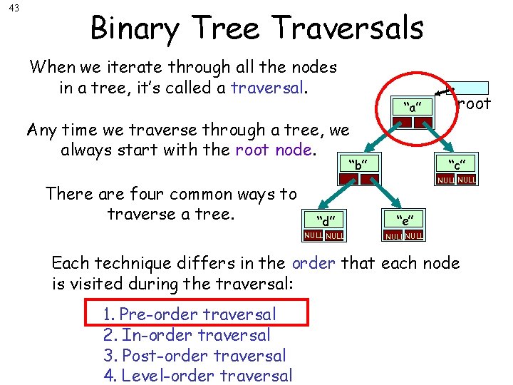
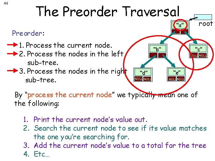
43 Binary Tree Traversals When we iterate through all the nodes in a tree, it’s called a traversal. “a” Any time we traverse through a tree, we always start with the root node. “c” “b” There are four common ways to traverse a tree. root NULL “d” “e” NULL Each technique differs in the order that each node is visited during the traversal: 1. Pre-order traversal 2. In-order traversal 3. Post-order traversal 4. Level-order traversal

44 The Preorder Traversal Preorder: 1. Process the current node. 2. Process the nodes in the left sub-tree. 3. Process the nodes in the right sub-tree. root “a” “c” “b” NULL “d” “e” NULL By “process the current node” we typically mean one of the following: 1. Print the current node’s value out. 2. Search the current node to see if its value matches the one you’re searching for. 3. Add the current node’s value to a total for the tree 4. Etc…

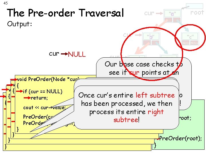
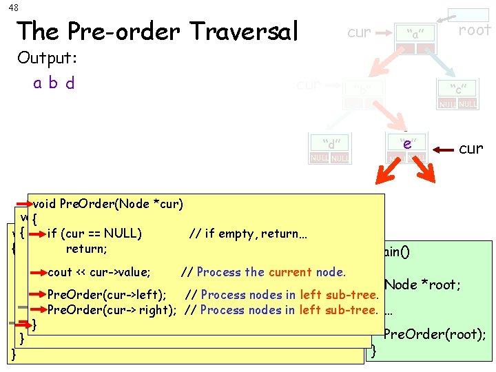
45 The Pre-order Traversal cur “a” a root Output: cur “b” b “c” NULL cur “e” “d” d NULLcase NULL Our base checks NULLto see if cur points at an void Pre. Order(Node *cur) empty sub-tree. void Pre. Order(Node *cur) { Otherwise we “process” void *cur) { Pre. Order(Node if (cur == NULL) //Then if empty, return… we usethere’s recursion to to If so, nothing Once cur’s entire left subtree { Pre. Order(Node void *cur) the value in the current if (cur == NULL) // if empty, return… return; process cur’s entire left == NULL) // if empty, return… { if (cur return; process and we’re done! has been processed, we then main() node… cout << cur->value; // Process the current node. return; if (cur == NULL) // if subtree empty, return… (a simplifying step). { process its entire right cout << cur->value; // Process the current node. return; // Process nodes innode. left sub-tree. Node *root; cout. Pre. Order(cur->left); << cur->value; // Process the current subtree! Pre. Order(cur->left); Pre. Order(cur-> right); ////Processnodesininleftsub-tree. } cout << cur->value; // Process the current node. Pre. Order(cur->left); nodes ininleft sub-tree. Process nodes left sub-tree. … }Pre. Order(cur-> right); ////Processnodesininleftsub-tree. Pre. Order(cur->left); }Pre. Order(cur-> right); ////Process Pre. Order(root); } Pre. Order(cur-> right); // Process nodes in left sub-tree. }

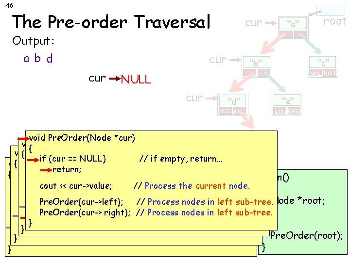
46 The Pre-order Traversal Output: a b d cur cur “a” root “c” “b” NULL cur “d” “e” NULL void Pre. Order(Node *cur) { void { Pre. Order(Node *cur) if (cur == NULL) // if empty, return… { Pre. Order(Node void *cur) if (cur == NULL) // if empty, return… return; == NULL) // if empty, return… { if (cur return; main() return; if (cur == NULL) return… cout << cur->value; // if//empty, Process the current node. { cout << cur->value; // Process the current node. return; cout. Pre. Order(cur->left); << cur->value; // Process the current // Process nodes innode. left sub-tree. Node *root; Pre. Order(cur->left); // Process in node. left sub-tree. cout << cur->value; right); // Process the nodes current Pre. Order(cur-> // Process nodes in left sub-tree. Pre. Order(cur->left); // Process nodes in left sub-tree. Pre. Order(cur-> right); // Process nodes in left sub-tree. … } Processnodesininleftsub-tree. Pre. Order(cur->left); }Pre. Order(cur-> right); ////Process Pre. Order(root); } Pre. Order(cur-> right); // Process nodes in left sub-tree. } }

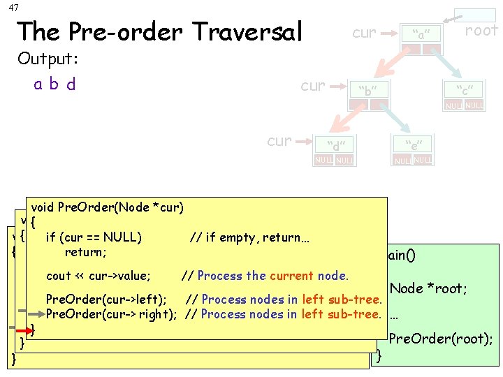
47 The Pre-order Traversal Output: a b d cur “a” root “c” “b” NULL cur “d” “e” NULL void Pre. Order(Node *cur) void { Pre. Order(Node *cur) { Pre. Order(Node void *cur) if (cur == NULL) // if empty, return… { if (cur return; main() return; if (cur == NULL) // if empty, return… { cout << cur->value; // Process the current node. return; Node *root; cout << cur->value; // Process the current node. Pre. Order(cur->left); // Process in node. left sub-tree. cout << cur->value; // Process the nodes current Pre. Order(cur->left); nodes ininleft sub-tree. Pre. Order(cur-> right); ////Process nodes left sub-tree. … Processnodesininleftsub-tree. Pre. Order(cur->left); }Pre. Order(cur-> right); ////Process Pre. Order(root); } Pre. Order(cur-> right); // Process nodes in left sub-tree. } }

48 The Pre-order Traversal Output: a b d cur “a” root “c” “b” NULL “d” NULL “e” e NULL cur void Pre. Order(Node *cur) void { Pre. Order(Node *cur) { Pre. Order(Node void *cur) if (cur == NULL) // if empty, return… { if (curreturn; main() return; if (cur == NULL) // if empty, return… { cout << cur->value; // Process the current node. return; Node *root; cout << cur->value; // Process the current node. // Process nodes innode. left sub-tree. cout. Pre. Order(cur->left); << cur->value; // Process the current Pre. Order(cur->left); Process nodes in in left sub-tree. Pre. Order(cur-> right); //// Process nodes left sub-tree. … Processnodesininleftsub-tree. Pre. Order(cur->left); }Pre. Order(cur-> right); ////Process Pre. Order(root); } Pre. Order(cur-> right); // Process nodes in left sub-tree. } }

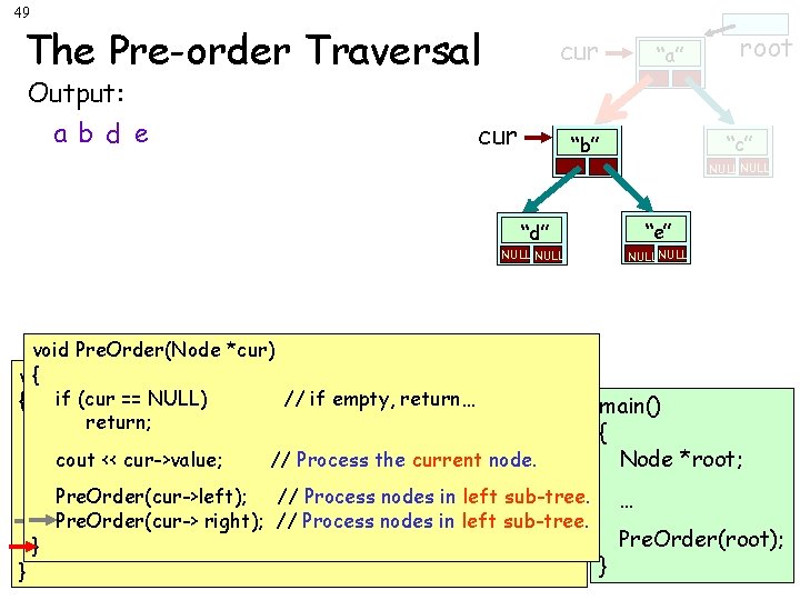
49 The Pre-order Traversal Output: a b d e cur “a” root “c” “b” NULL “d” “e” NULL void Pre. Order(Node *cur) { Pre. Order(Node *cur) void // if empty, return… { if (cur == NULL) main() return; if (cur == NULL) // if empty, return… { return; Node *root; cout << cur->value; // Process the current node. Pre. Order(cur->left); // Process nodes in left sub-tree. … Pre. Order(cur-> right); ////Processnodesininleftsub-tree. Pre. Order(cur->left); Pre. Order(root); } Pre. Order(cur-> right); // Process nodes in left sub-tree. } }

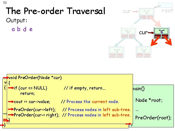
50 The Pre-order Traversal cur Output: a b d e “b” “a” cur “d” “e” NULL root “c” c NULL void Pre. Order(Node *cur) void { Pre. Order(Node *cur) { if (cur == NULL) // if empty, return… main() if (curreturn; == NULL) // if empty, return… { return; Node *root; cout << cur->value; // Process the current node. Pre. Order(cur->left); // Process nodes in left sub-tree. … Pre. Order(cur->left); Process nodes in in left sub-tree. Pre. Order(cur-> right); //// Process nodes left sub-tree. Pre. Order(root); }Pre. Order(cur-> right); // Process nodes in left sub-tree. } }