1 Inventory Management and Control 2 Inventory Defined

1 Inventory Management and Control

2 Inventory Defined • Inventory is the stock of any item or resource held to meet future demand can include: raw materials, finished products, component parts, supplies, and work-in-process

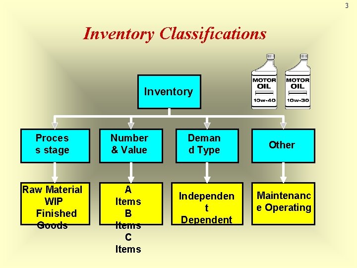
3 Inventory Classifications Inventory Proces s stage Number & Value Raw Material WIP Finished Goods A Items B Items C Items Deman d Type Independen t Dependent Other Maintenanc e Operating

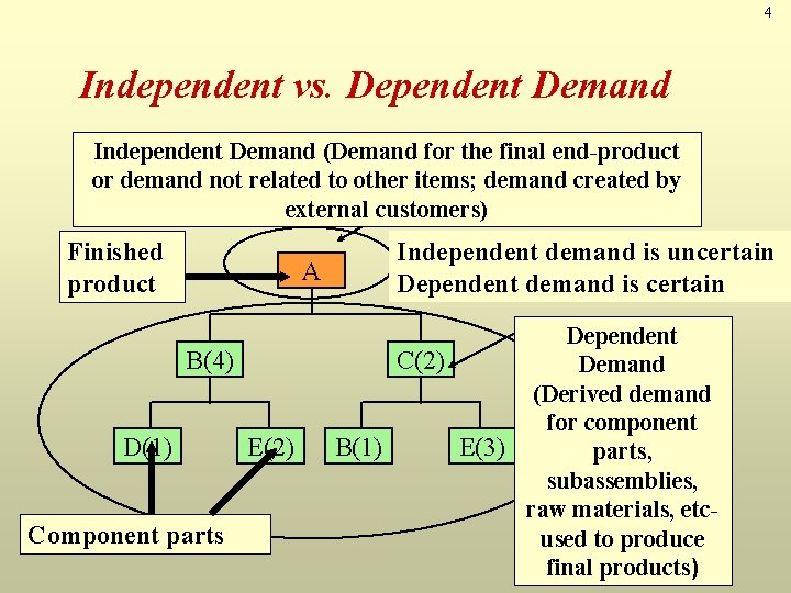
4 Independent vs. Dependent Demand Independent Demand (Demand for the final end-product or demand not related to other items; demand created by external customers) Finished product A B(4) D(1) Component parts E(1) E(2) Independent demand is uncertain Dependent demand is certain Dependent C(2) Demand (Derived demand for component B(1) E(3) parts, subassemblies, raw materials, etcused to produce final products)

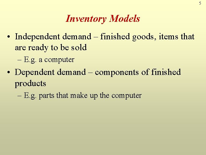
5 Inventory Models • Independent demand – finished goods, items that are ready to be sold – E. g. a computer • Dependent demand – components of finished products – E. g. parts that make up the computer

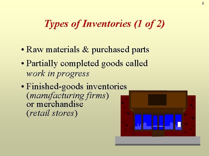
6 Types of Inventories (1 of 2) • Raw materials & purchased parts • Partially completed goods called work in progress • Finished-goods inventories (manufacturing firms) or merchandise (retail stores)

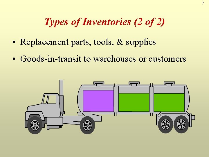
7 Types of Inventories (2 of 2) • Replacement parts, tools, & supplies • Goods-in-transit to warehouses or customers

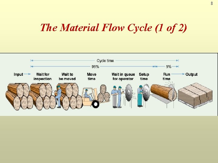
8 The Material Flow Cycle (1 of 2)

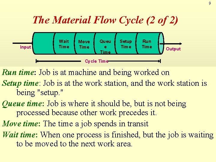
9 The Material Flow Cycle (2 of 2) Input Wait Time Move Time Queu e Time Setup Time Run Time Output Cycle Time Run time: Job is at machine and being worked on Setup time: Job is at the work station, and the work station is being "setup. " Queue time: Job is where it should be, but is not being processed because other work precedes it. Move time: The time a job spends in transit Wait time: When one process is finished, but the job is waiting to be moved to the next work area.

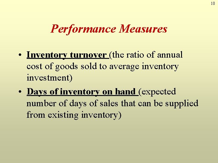
10 Performance Measures • Inventory turnover (the ratio of annual cost of goods sold to average inventory investment) • Days of inventory on hand (expected number of days of sales that can be supplied from existing inventory)

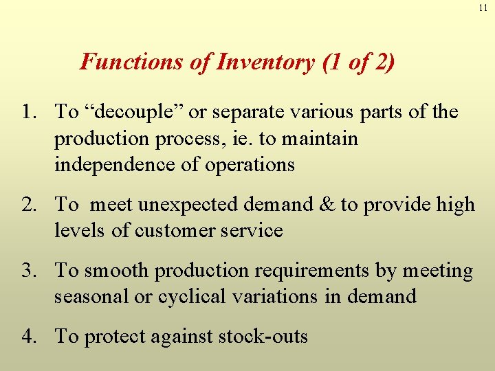
11 Functions of Inventory (1 of 2) 1. To “decouple” or separate various parts of the production process, ie. to maintain independence of operations 2. To meet unexpected demand & to provide high levels of customer service 3. To smooth production requirements by meeting seasonal or cyclical variations in demand 4. To protect against stock-outs

12 Functions of Inventory (2 of 2) 5. To provide a safeguard for variation in raw material delivery time 6. To provide a stock of goods that will provide a “selection” for customers 7. To take advantage of economic purchase-order size 8. To take advantage of quantity discounts 9. To hedge against price increases

13 Disadvantages of Inventory • Higher costs – Item cost (if purchased) – Holding (or carrying) cost • Difficult to control • Hides production problems • May decrease flexibility

14 Inventory Costs Ø Holding (or carrying) costs § Costs for storage, handling, insurance, etc Ø Setup (or production change) costs § Costs to prepare a machine or process for manufacturing an order, eg. arranging specific equipment setups, etc Ø Ordering costs (costs of replenishing inventory) § Costs of placing an order and receiving goods Ø Shortage costs § Costs incurred when demand exceeds supply

15 Holding (Carrying) Costs • • Obsolescence Insurance Extra staffing Interest Pilferage Damage Warehousing Etc.

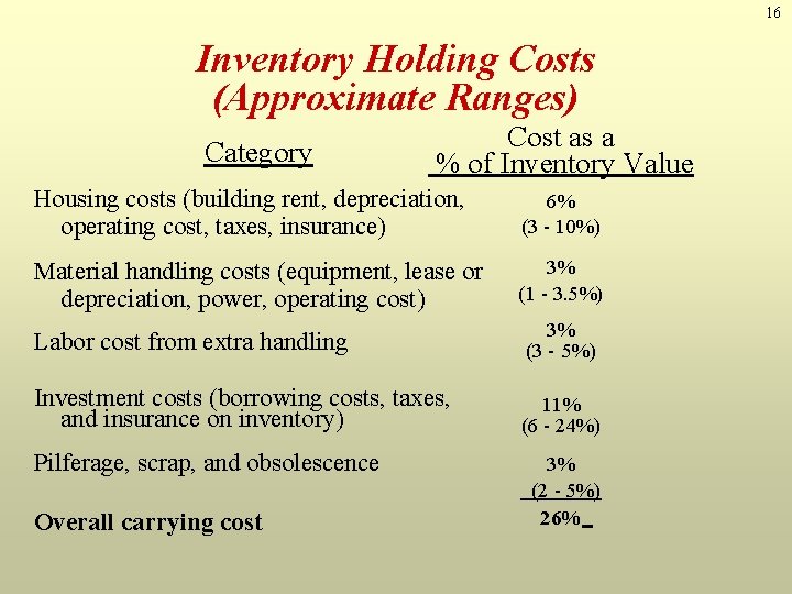
16 Inventory Holding Costs (Approximate Ranges) Category Cost as a % of Inventory Value Housing costs (building rent, depreciation, operating cost, taxes, insurance) 6% (3 - 10%) Material handling costs (equipment, lease or depreciation, power, operating cost) 3% (1 - 3. 5%) Labor cost from extra handling 3% (3 - 5%) Investment costs (borrowing costs, taxes, and insurance on inventory) 11% (6 - 24%) Pilferage, scrap, and obsolescence Overall carrying cost 3% (2 - 5%) 26%

17 Ordering Costs • • • Supplies Forms Order processing Clerical support etc.

18 Setup Costs • • Clean-up costs Re-tooling costs Adjustment costs etc.

19 Shortage Costs • Backordering cost • Cost of lost sales

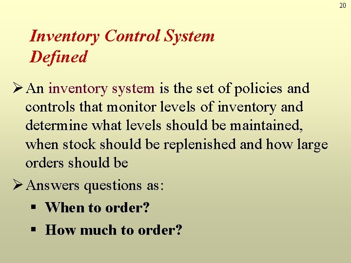
20 Inventory Control System Defined Ø An inventory system is the set of policies and controls that monitor levels of inventory and determine what levels should be maintained, when stock should be replenished and how large orders should be Ø Answers questions as: § When to order? § How much to order?

21 Objective of Inventory Control To achieve satisfactory levels of customer service while keeping inventory costs within reasonable bounds ØImprove the Level of customer service ØReduce the Costs of ordering and carrying inventory

22 Requirements of an Effective Inventory Management ØA system to keep track of inventory ØA reliable forecast of demand ØKnowledge of lead times ØReasonable estimates of § Holding costs § Ordering costs § Shortage costs ØA classification system

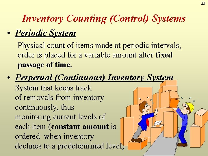
23 Inventory Counting (Control) Systems • Periodic System Physical count of items made at periodic intervals; order is placed for a variable amount after fixed passage of time. • Perpetual (Continuous) Inventory System that keeps track of removals from inventory continuously, thus monitoring current levels of each item (constant amount is ordered when inventory declines to a predetermined level)

24 Inventory Models Ø Single-Period Inventory Model § One time purchasing decision (Examples: selling tshirts at a football game, newspapers, fresh bakery products, fresh flowers) § Seeks to balance the costs of inventory over stock and under stock Ø Multi-Period Inventory Models § Fixed-Order Quantity Models • Event triggered (Example: running out of stock) § Fixed-Time Period Models • Time triggered (Example: Monthly sales call by

25 Single-Period Inventory Model

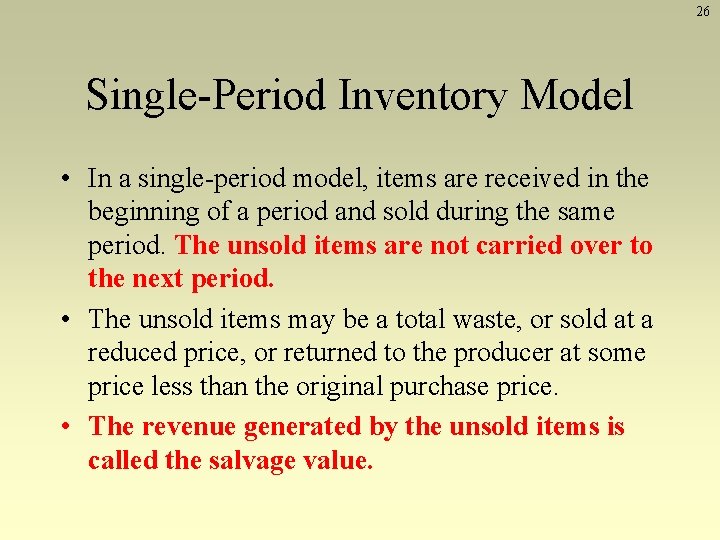
26 Single-Period Inventory Model • In a single-period model, items are received in the beginning of a period and sold during the same period. The unsold items are not carried over to the next period. • The unsold items may be a total waste, or sold at a reduced price, or returned to the producer at some price less than the original purchase price. • The revenue generated by the unsold items is called the salvage value.

3 (Newsboy Problem) • Single period model: It is used to handle ordering of perishables (fresh fruits, flowers) and other items with limited useful lives (newspapers, spare parts for specialized equipment). 27

28 Shortage cost (Cost of Understocking) • Shortage cost: generally, this cost represents unrealized profit per unit (Cu=Revenue per unit – Cost per unit) • If a shortage or stockout cost relates to a spare part for a machine, then shortage cost refers to the actual cost of lost production.

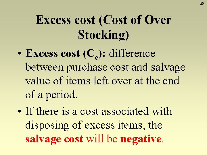
29 Excess cost (Cost of Over Stocking) • Excess cost (Ce): difference between purchase cost and salvage value of items left over at the end of a period. • If there is a cost associated with disposing of excess items, the salvage cost will be negative.

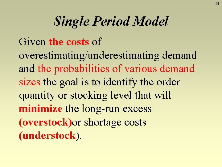
30 Single Period Model Given the costs of overestimating/underestimating demand the probabilities of various demand sizes the goal is to identify the order quantity or stocking level that will minimize the long-run excess (overstock)or shortage costs (understock).

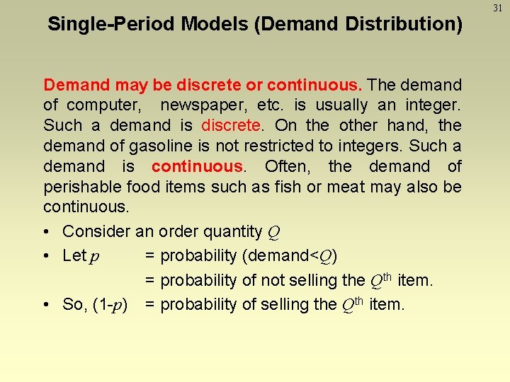
Single-Period Models (Demand Distribution) Demand may be discrete or continuous. The demand of computer, newspaper, etc. is usually an integer. Such a demand is discrete. On the other hand, the demand of gasoline is not restricted to integers. Such a demand is continuous. Often, the demand of perishable food items such as fish or meat may also be continuous. • Consider an order quantity Q • Let p = probability (demand<Q) = probability of not selling the Qth item. • So, (1 -p) = probability of selling the Qth item. 31

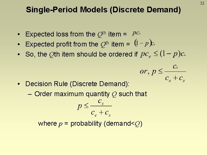
Single-Period Models (Discrete Demand) • Expected loss from the Qth item = • Expected profit from the Qth item = • So, the Qth item should be ordered if • Decision Rule (Discrete Demand): – Order maximum quantity Q such that where p = probability (demand<Q) 32

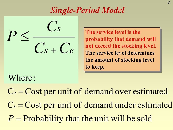
33 Single-Period Model The service level is the probability that demand will not exceed the stocking level. The service level determines the amount of stocking level to keep.

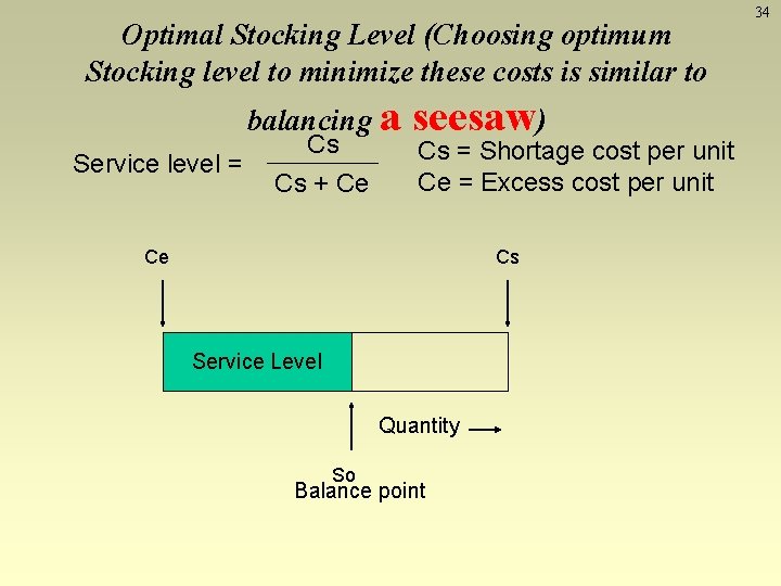
Optimal Stocking Level (Choosing optimum Stocking level to minimize these costs is similar to balancing a Service level = Cs Cs + Ce seesaw) Cs = Shortage cost per unit Ce = Excess cost per unit Ce Cs Service Level Quantity So Balance point 34

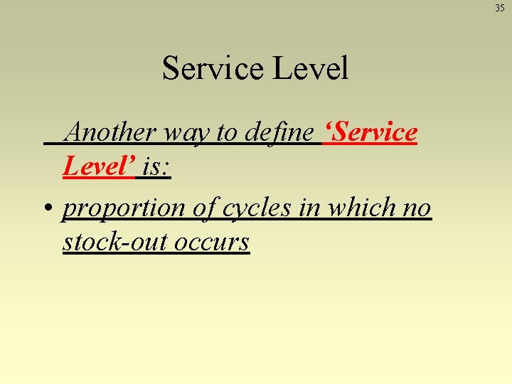
35 Service Level Another way to define ‘Service Level’ is: • proportion of cycles in which no stock-out occurs

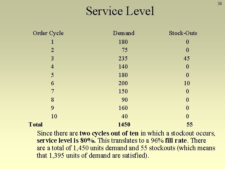
36 Service Level Order Cycle 1 2 3 4 5 6 7 8 9 10 Total Demand 180 75 235 140 180 200 150 90 160 40 1450 Stock-Outs 0 0 45 0 0 10 0 0 55 Since there are two cycles out of ten in which a stockout occurs, service level is 80%. This translates to a 96% fill rate. There a total of 1, 450 units demand 55 stockouts (which means that 1, 395 units of demand are satisfied).

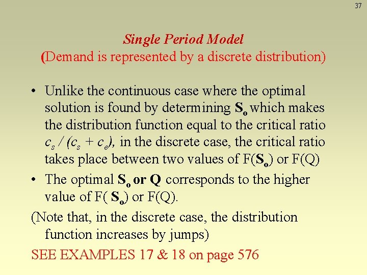
37 Single Period Model (Demand is represented by a discrete distribution) • Unlike the continuous case where the optimal solution is found by determining So which makes the distribution function equal to the critical ratio cs / (cs + ce), in the discrete case, the critical ratio takes place between two values of F(So) or F(Q) • The optimal So or Q corresponds to the higher value of F( So) or F(Q). (Note that, in the discrete case, the distribution function increases by jumps) SEE EXAMPLES 17 & 18 on page 576

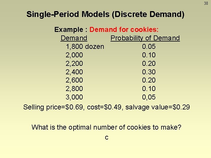
38 Single-Period Models (Discrete Demand) Example : Demand for cookies: Demand Probability of Demand 1, 800 dozen 0. 05 2, 000 0. 10 2, 200 0. 20 2, 400 0. 30 2, 600 0. 20 2, 800 0. 10 3, 000 0, 05 Selling price=$0. 69, cost=$0. 49, salvage value=$0. 29 What is the optimal number of cookies to make? c

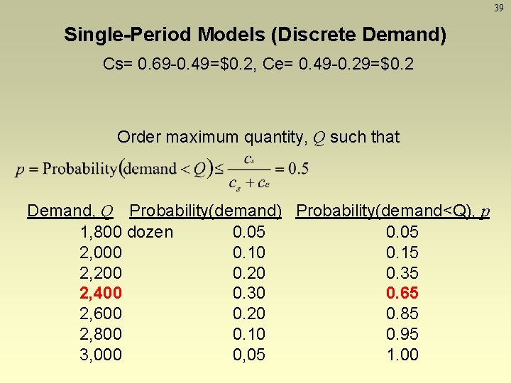
39 Single-Period Models (Discrete Demand) Cs= 0. 69 -0. 49=$0. 2, Ce= 0. 49 -0. 29=$0. 2 Order maximum quantity, Q such that Demand, Q Probability(demand) Probability(demand<Q), p 1, 800 dozen 0. 05 2, 000 0. 15 2, 200 0. 20 0. 35 2, 400 0. 30 0. 65 2, 600 0. 20 0. 85 2, 800 0. 10 0. 95 3, 000 0, 05 1. 00

40 Single-Period Models (Continous Demand) • Often the demand is continuous. Even when the demand is not continuous, continuous distribution may be used because the discrete distribution may be inconvenient. • We shall discuss two distributions: Uniform distribution Normal distribution

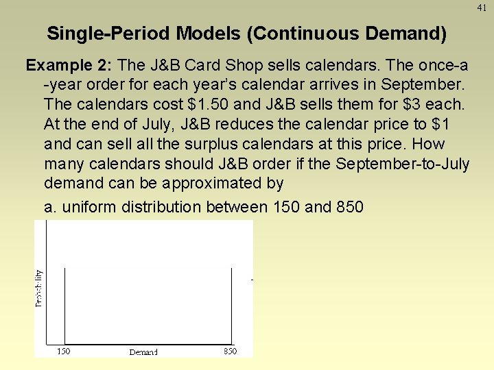
41 Single-Period Models (Continuous Demand) Example 2: The J&B Card Shop sells calendars. The once-a -year order for each year’s calendar arrives in September. The calendars cost $1. 50 and J&B sells them for $3 each. At the end of July, J&B reduces the calendar price to $1 and can sell all the surplus calendars at this price. How many calendars should J&B order if the September-to-July demand can be approximated by a. uniform distribution between 150 and 850

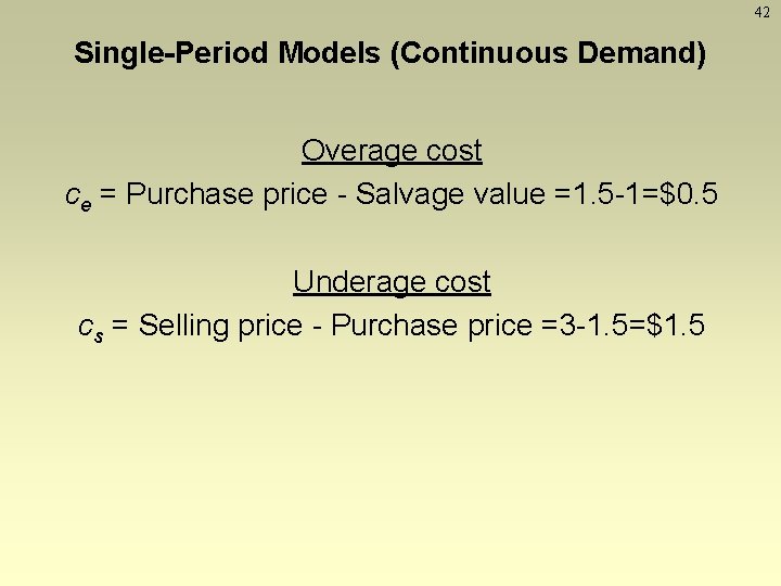
42 Single-Period Models (Continuous Demand) Overage cost ce = Purchase price - Salvage value =1. 5 -1=$0. 5 Underage cost cs = Selling price - Purchase price =3 -1. 5=$1. 5

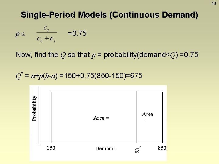
43 Single-Period Models (Continuous Demand) =0. 75 p Now, find the Q so that p = probability(demand<Q) =0. 75 Probability Q* = a+p(b-a) =150+0. 75(850 -150)=675 Area = 150 Demand Q* 850

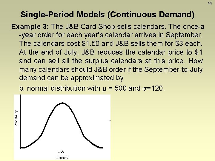
44 Single-Period Models (Continuous Demand) Example 3: The J&B Card Shop sells calendars. The once-a -year order for each year’s calendar arrives in September. The calendars cost $1. 50 and J&B sells them for $3 each. At the end of July, J&B reduces the calendar price to $1 and can sell all the surplus calendars at this price. How many calendars should J&B order if the September-to-July demand can be approximated by b. normal distribution with = 500 and =120.

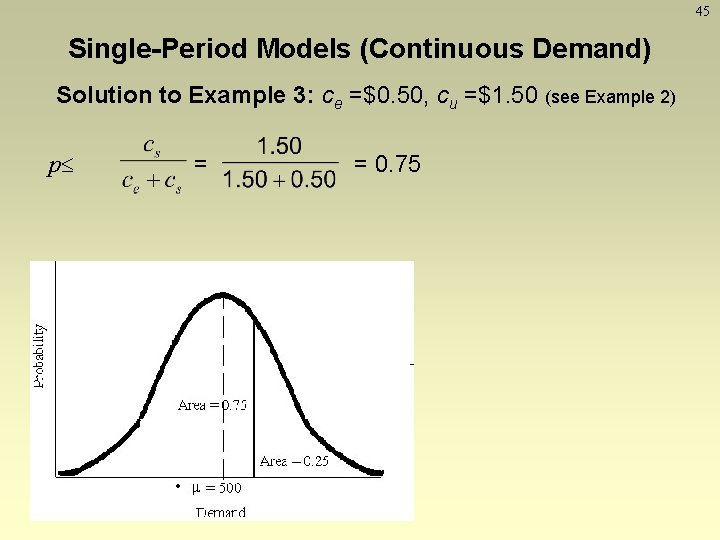
45 Single-Period Models (Continuous Demand) Solution to Example 3: ce =$0. 50, cu =$1. 50 (see Example 2) p = = 0. 75

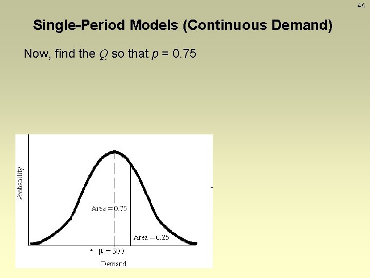
46 Single-Period Models (Continuous Demand) Now, find the Q so that p = 0. 75

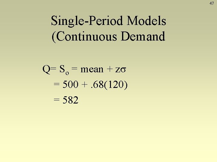
47 Single-Period Models (Continuous Demand Q= So = mean + zσ = 500 +. 68(120) = 582

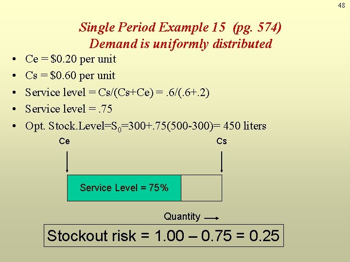
48 Single Period Example 15 (pg. 574) Demand is uniformly distributed • • • Ce = $0. 20 per unit Cs = $0. 60 per unit Service level = Cs/(Cs+Ce) =. 6/(. 6+. 2) Service level =. 75 Opt. Stock. Level=S 0=300+. 75(500 -300)= 450 liters Ce Cs Service Level = 75% Quantity Stockout risk = 1. 00 – 0. 75 = 0. 25

49 Uniform Distribution [Continuous Dist’n] • A random variable X is uniformly distributed on the interval (a, b), U(a, b), if its pdf and cdf are: • Properties – P(x 1 < X < x 2) is proportional to the length of the interval [F(x 2) – F(x 1) = (x 2 -x 1)/(b-a)] – E(X) = (a+b)/2 V(X) = (b-a)2/12 • U(0, 1) provides the means to generate random numbers, from which random variates can be generated. 49

50 Poisson Distribution [Discrete Dist’n] • Poisson distribution describes many random processes quite well and is mathematically quite simple. – where a > 0, pdf and cdf are: – E(X) = a = V(X) 50

51 Normal Distribution [Continuous Dist’n] • A normally distributed random variable X has the pdf: – Mean: – Variance: – Denoted as X ~ N(m, s 2) • Special properties: . – symmetric about m. – The maximum value of the pdf occurs at x = m; the mean and mode are equal. 51

52 Normal Distribution [Continuous Dist’n] • Evaluating the distribution: – Use numerical methods (no closed form) – Independent of and , using the standard normal distribution: Z ~ N(0, 1) – Transformation of variables: let Z = (X - m) / s, 52

53 Normal Distribution [Continuous Dist’n] • Example: The time required to load an oceangoing vessel, X, is distributed as N(12, 4) – The probability that the vessel is loaded in less than 10 hours: • Using the symmetry property, F(1) is the complement of F (-1) 53

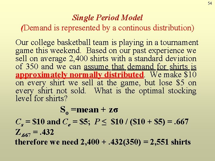
54 Single Period Model (Demand is represented by a continous distribution) Our college basketball team is playing in a tournament game this weekend. Based on our past experience we sell on average 2, 400 shirts with a standard deviation of 350 and we can assume that demand for shirts is approximately normally distributed. We make $10 on every shirt we sell at the game, but lose $5 on every shirt not sold. What is the optimal stocking level for shirts? So =mean + zσ Cs = $10 and Ce = $5; P ≤ $10 / ($10 + $5) =. 667 Z. 667 =. 432 therefore we need 2, 400 +. 432(350) = 2, 551 shirts

55 Multi-Period Inventory Models ØFixed-Order Quantity Models (Types of) üEconomic Order Quantity Model (EOQ) üEconomic Production Order Quantity (Economic Lot Size) Model (EPQ) üEconomic Order Quantity Model with Quantity Discounts ØFixed Time Period (Fixed Order Interval) Models

56 Fixed Order Quantity Models: Economic Order Quantity Model

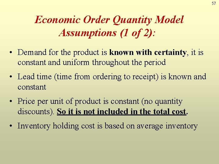
57 Economic Order Quantity Model Assumptions (1 of 2): • Demand for the product is known with certainty, it is constant and uniform throughout the period • Lead time (time from ordering to receipt) is known and constant • Price per unit of product is constant (no quantity discounts). So it is not included in the total cost. • Inventory holding cost is based on average inventory

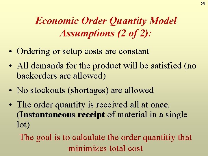
58 Economic Order Quantity Model Assumptions (2 of 2): • Ordering or setup costs are constant • All demands for the product will be satisfied (no backorders are allowed) • No stockouts (shortages) are allowed • The order quantity is received all at once. (Instantaneous receipt of material in a single lot) The goal is to calculate the order quantitiy that minimizes total cost

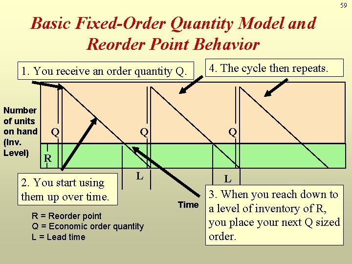
59 Basic Fixed-Order Quantity Model and Reorder Point Behavior 1. You receive an order quantity Q. Number of units on hand (Inv. Level) Q Q 4. The cycle then repeats. Q R 2. You start using them up over time. L R = Reorder point Q = Economic order quantity L = Lead time Time L 3. When you reach down to a level of inventory of R, you place your next Q sized order.

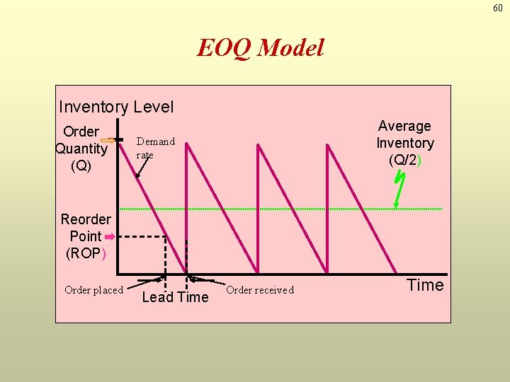
60 EOQ Model Inventory Level Order Quantity (Q) Average Inventory (Q/2) Demand rate Reorder Point (ROP) Order placed Lead Time Order received Time

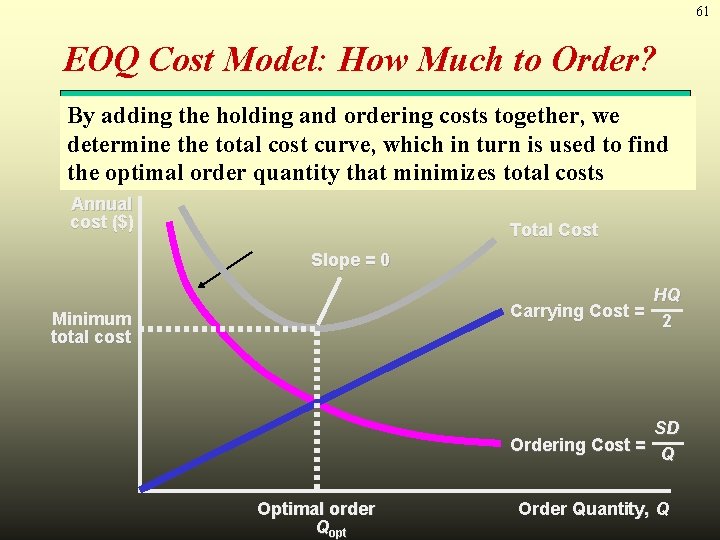
61 EOQ Cost Model: How Much to Order? By adding the holding and ordering costs together, we determine the total cost curve, which in turn is used to find the optimal order quantity that minimizes total costs Annual cost ($) Total Cost Slope = 0 HQ Carrying Cost = 2 Minimum total cost SD Ordering Cost = Q Optimal order Qopt Order Quantity, Q

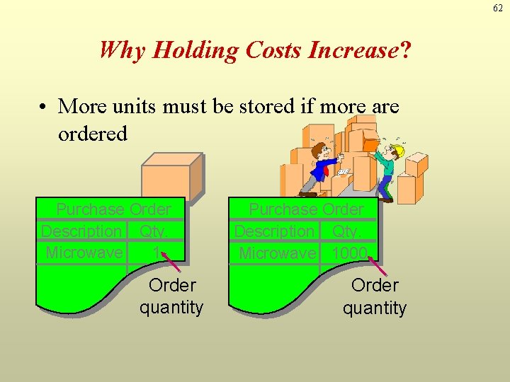
62 Why Holding Costs Increase? • More units must be stored if more are ordered Purchase Order Description Qty. Microwave 1 Order quantity Purchase Order Description Qty. Microwave 1000 Order quantity

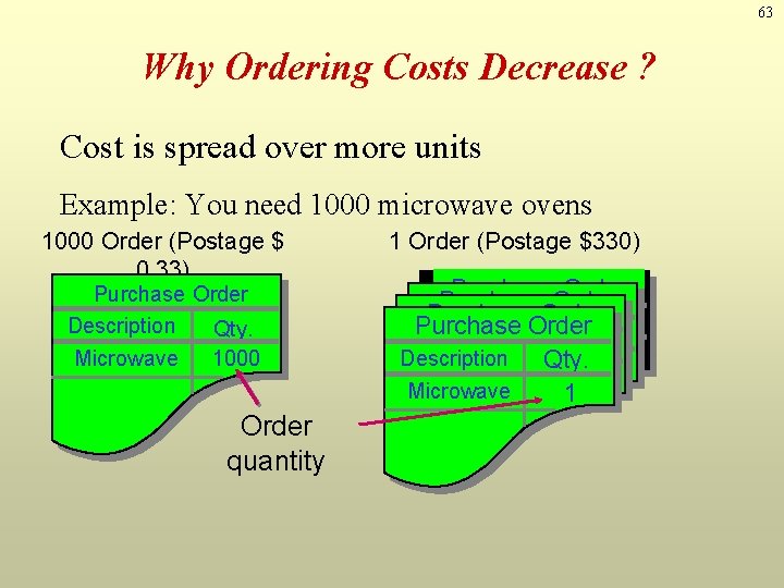
63 Why Ordering Costs Decrease ? Cost is spread over more units Example: You need 1000 microwave ovens 1000 Order (Postage $ 0. 33) Purchase Order Description Qty. Microwave 1000 Order quantity 1 Order (Postage $330) Purchase. Order Description Qty. Purchase Description Qty. 1 Microwave Description Qty. Microwave 11 Microwave 1

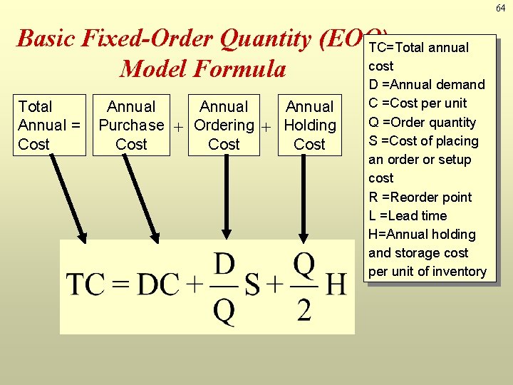
64 Basic Fixed-Order Quantity (EOQ) TC=Total annual cost Model Formula D =Annual demand Total Annual = Cost Annual Purchase + Ordering + Holding Cost C =Cost per unit Q =Order quantity S =Cost of placing an order or setup cost R =Reorder point L =Lead time H=Annual holding and storage cost per unit of inventory

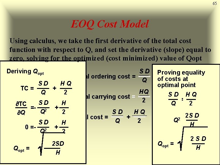
65 EOQ Cost Model Using calculus, we take the first derivative of the total cost function with respect to Q, and set the derivative (slope) equal to zero, solving for the optimized (cost minimized) value of Qopt Deriving Qopt SD Annual ordering cost = Q SD HQ TC = + HQ Q 2 Annual carrying cost = 2 SD H TC =- 2 + Q 2 SD HQ Q Total cost = + Q 2 SD H 0 =- 2 + Q 2 Qopt = 2 SD H Proving equality of costs at optimal point SD HQ = Q 2 2 S D Q 2 = H Qopt = 2 SD H

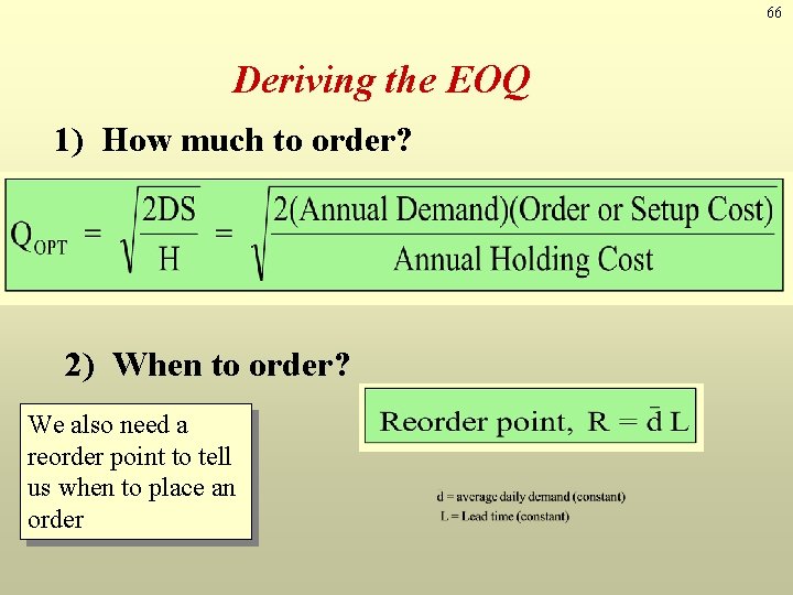
66 Deriving the EOQ 1) How much to order? 2) When to order? We also need a reorder point to tell us when to place an order

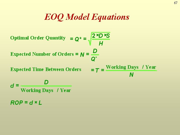
67 EOQ Model Equations 2 ×D ×S H D Expected Number of Orders = N = Q* Optimal Order Quantity = Q* = Expected Time Between Orders d= D Working Days / Year ROP = d × L =T = Working Days / Year N

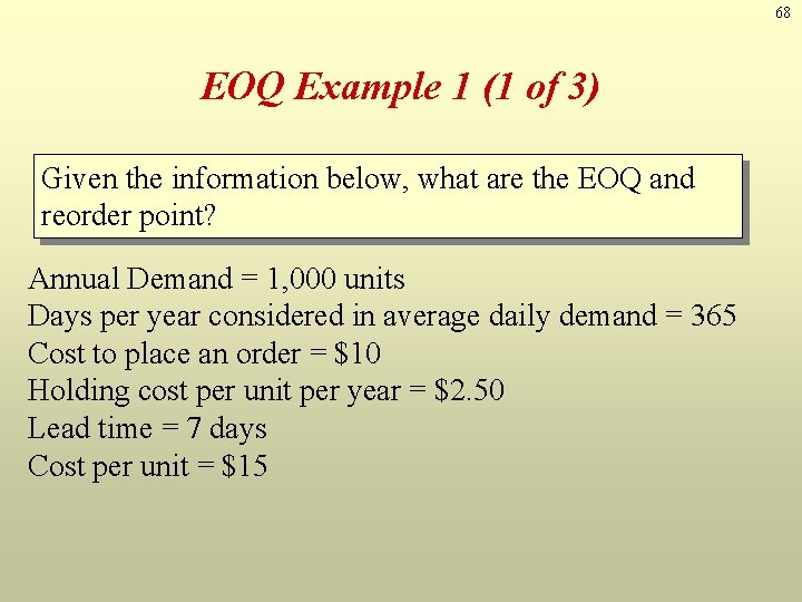
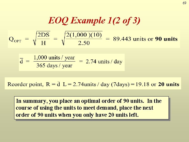
68 EOQ Example 1 (1 of 3) Given the information below, what are the EOQ and reorder point? Annual Demand = 1, 000 units Days per year considered in average daily demand = 365 Cost to place an order = $10 Holding cost per unit per year = $2. 50 Lead time = 7 days Cost per unit = $15

69 EOQ Example 1(2 of 3) In summary, you place an optimal order of 90 units. In the course of using the units to meet demand, place the next order of 90 units when you only have 20 units left.

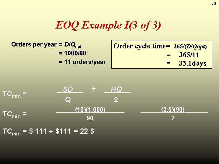
70 EOQ Example I(3 of 3) Orders per year = D/Qopt = 1000/90 = 11 orders/year TCmin = SD Q + (10)(1, 000) 90 TCmin = $ 111 + $111 = 22 $ Order cycle time= 365/(D/Qopt) = 365/11 = 33. 1 days HQ 2 + (2, 5)(90) 2

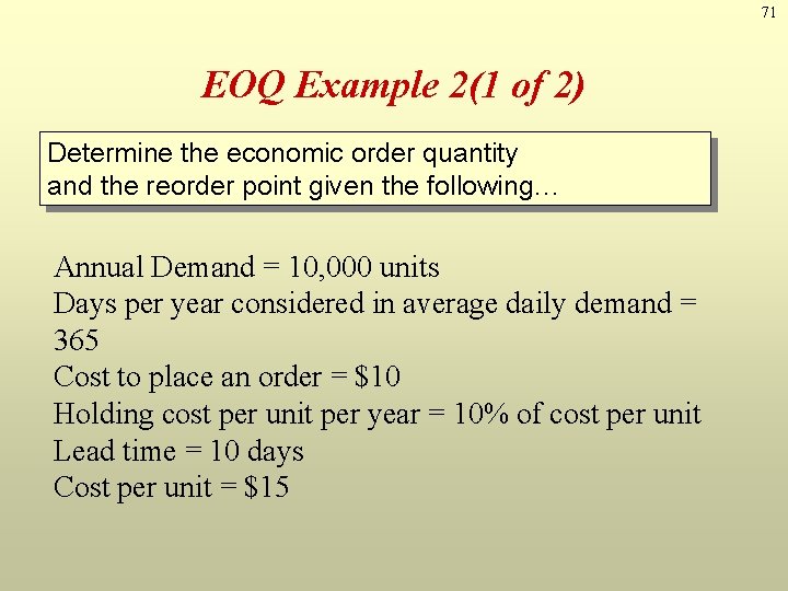
71 EOQ Example 2(1 of 2) Determine the economic order quantity and the reorder point given the following… Annual Demand = 10, 000 units Days per year considered in average daily demand = 365 Cost to place an order = $10 Holding cost per unit per year = 10% of cost per unit Lead time = 10 days Cost per unit = $15

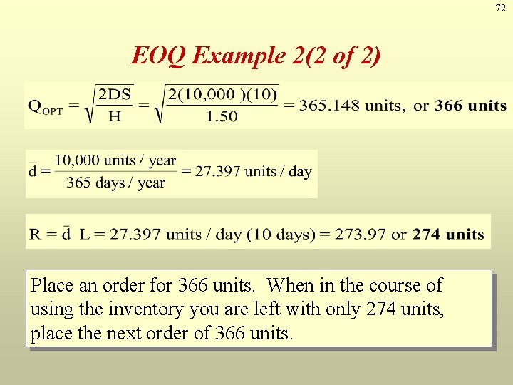
72 EOQ Example 2(2 of 2) Place an order for 366 units. When in the course of using the inventory you are left with only 274 units, place the next order of 366 units.

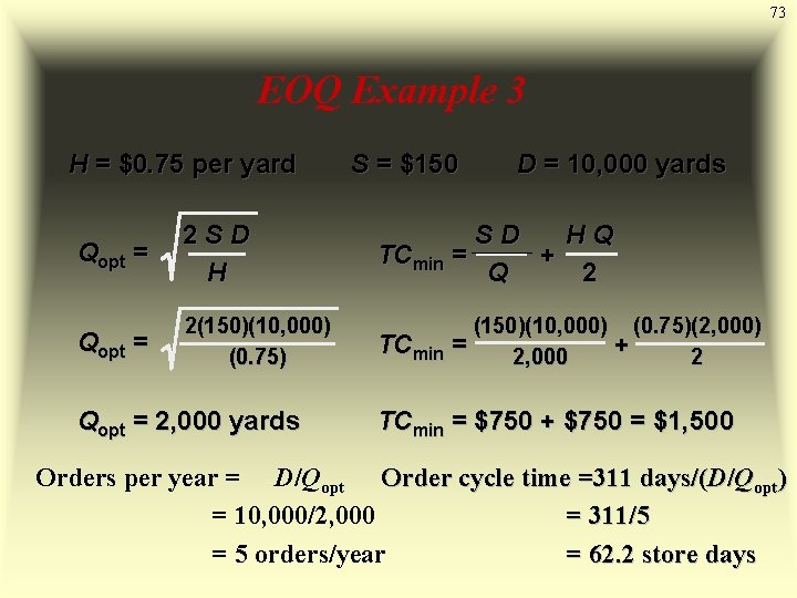
73 EOQ Example 3 H = $0. 75 per yard Qopt = 2 SD H Qopt = 2(150)(10, 000) (0. 75) Qopt = 2, 000 yards S = $150 D = 10, 000 yards SD HQ TCmin = + Q 2 TCmin (150)(10, 000) (0. 75)(2, 000) = + 2, 000 2 TCmin = $750 + $750 = $1, 500 Orders per year = D/Qopt Order cycle time =311 days/(D/Qopt) = 10, 000/2, 000 = 311/5 = 5 orders/year = 62. 2 store days

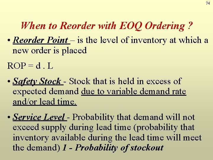
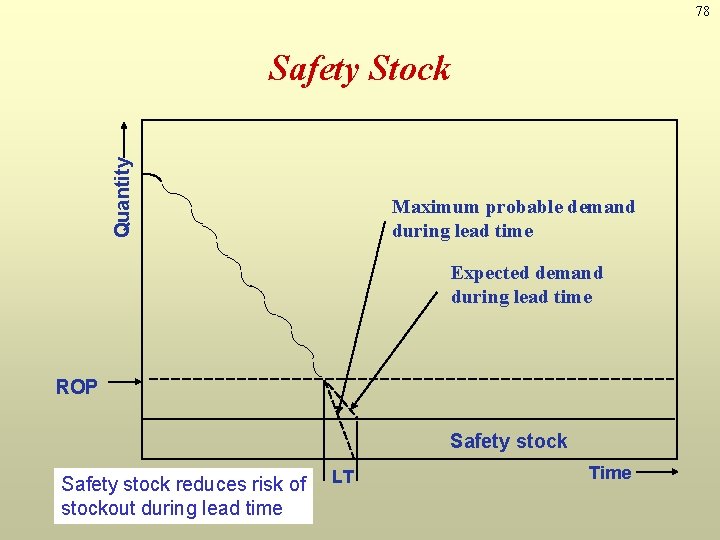
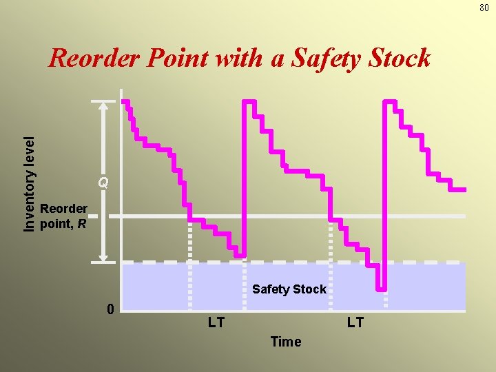
74 When to Reorder with EOQ Ordering ? • Reorder Point – is the level of inventory at which a new order is placed ROP = d. L • Safety Stock - Stock that is held in excess of expected demand due to variable demand rate and/or lead time. • Service Level - Probability that demand will not exceed supply during lead time (probability that inventory available during the lead time will meet the demand) 1 - Probability of stockout

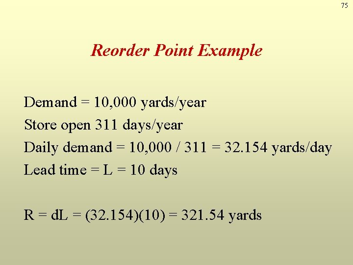
75 Reorder Point Example Demand = 10, 000 yards/year Store open 311 days/year Daily demand = 10, 000 / 311 = 32. 154 yards/day Lead time = L = 10 days R = d. L = (32. 154)(10) = 321. 54 yards

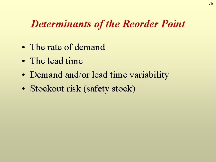
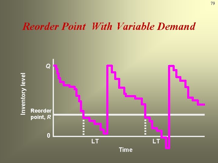
76 Determinants of the Reorder Point • • The rate of demand The lead time Demand and/or lead time variability Stockout risk (safety stock)

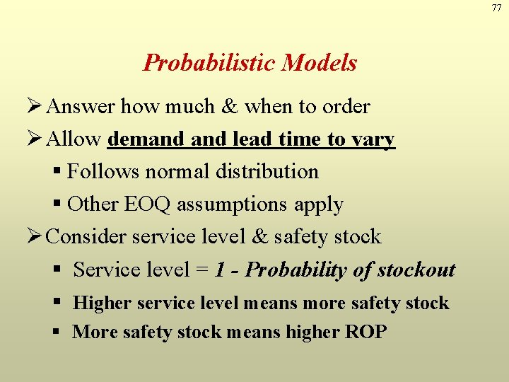
77 Probabilistic Models Ø Answer how much & when to order Ø Allow demand lead time to vary § Follows normal distribution § Other EOQ assumptions apply Ø Consider service level & safety stock § Service level = 1 - Probability of stockout § Higher service level means more safety stock § More safety stock means higher ROP

78 Quantity Safety Stock Maximum probable demand during lead time Expected demand during lead time ROP Safety stock reduces risk of stockout during lead time LT Time

79 Reorder Point With Variable Demand Inventory level Q Reorder point, R 0 LT LT Time

80 Inventory level Reorder Point with a Safety Stock Q Reorder point, R Safety Stock 0 LT LT Time

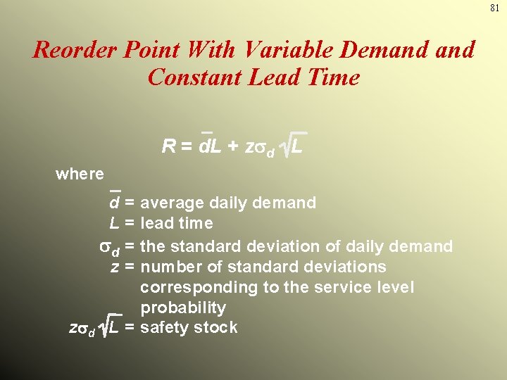
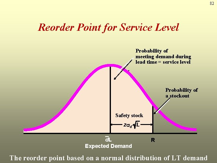
81 Reorder Point With Variable Demand Constant Lead Time R = d. L + z d L where d = average daily demand L = lead time d = the standard deviation of daily demand z = number of standard deviations corresponding to the service level probability z d L = safety stock

82 Reorder Point for Service Level Probability of meeting demand during lead time = service level Probability of a stockout Safety stock z d L d. L Expected Demand R The reorder point based on a normal distribution of LT demand

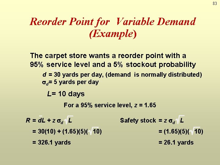
83 Reorder Point for Variable Demand (Example) The carpet store wants a reorder point with a 95% service level and a 5% stockout probability d = 30 yards per day, (demand is normally distributed) d = 5 yards per day L= 10 days For a 95% service level, z = 1. 65 R = d. L + z d L Safety stock = z d L = 30(10) + (1. 65)(5)( 10) = 326. 1 yards = 26. 1 yards

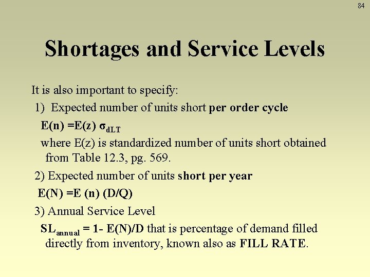
84 Shortages and Service Levels It is also important to specify: 1) Expected number of units short per order cycle E(n) =E(z) σd. LT where E(z) is standardized number of units short obtained from Table 12. 3, pg. 569. 2) Expected number of units short per year E(N) =E (n) (D/Q) 3) Annual Service Level SLannual = 1 - E(N)/D that is percentage of demand filled directly from inventory, known also as FILL RATE.

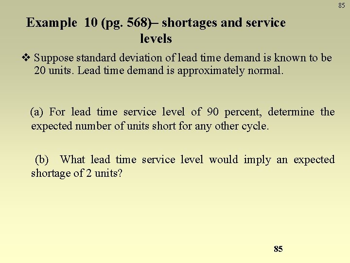
85 Example 10 (pg. 568)– shortages and service levels v Suppose standard deviation of lead time demand is known to be 20 units. Lead time demand is approximately normal. (a) For lead time service level of 90 percent, determine the expected number of units short for any other cycle. (b) What lead time service level would imply an expected shortage of 2 units? 85

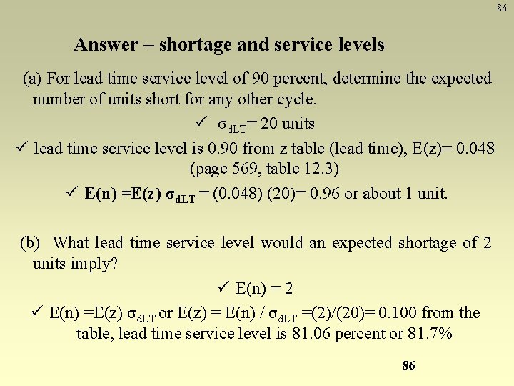
86 Answer – shortage and service levels (a) For lead time service level of 90 percent, determine the expected number of units short for any other cycle. ü σd. LT= 20 units ü lead time service level is 0. 90 from z table (lead time), E(z)= 0. 048 (page 569, table 12. 3) ü E(n) =E(z) σd. LT = (0. 048) (20)= 0. 96 or about 1 unit. (b) What lead time service level would an expected shortage of 2 units imply? ü E(n) = 2 ü E(n) =E(z) σd. LT or E(z) = E(n) / σd. LT =(2)/(20)= 0. 100 from the table, lead time service level is 81. 06 percent or 81. 7% 86

87 Shortages and Service Levels • Expected number of units short per year See example 11, page 568 • Annual Service Level See example 12, page 570 Note that annual service level will usually be grater than the cycle service level

88 Fixed Order Quantity Models: -Noninstantaneous Receipt. Production Order Quantity (Economic Lot Size) Model

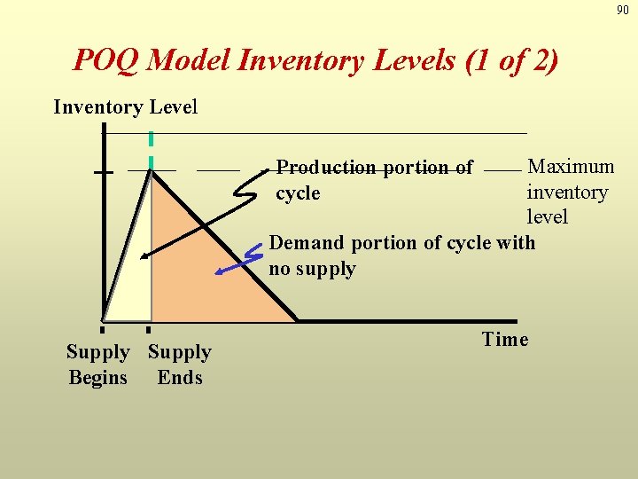
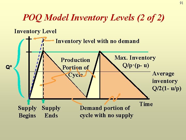
89 Production Order Quantity Model Ø Production done in batches or lots Ø Capacity to produce a part exceeds that part’s usage or demand rate Ø Allows partial receipt of material § Other EOQ assumptions apply Ø Suited for production environment § Material produced, used immediately § Provides production lot size Ø Lower holding cost than EOQ model Ø Answers how much to order and when to order

90 POQ Model Inventory Levels (1 of 2) Inventory Level Maximum inventory level Demand portion of cycle with no supply Production portion of cycle Supply Begins Ends Time

91 POQ Model Inventory Levels (2 of 2) Inventory Level Inventory level with no demand Production Portion of Cycle Q* Supply Begins Ends Max. Inventory Q/p·(p- u) Average inventory Q/2(1 - u/p) Demand portion of cycle with no supply Time

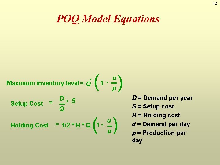
92 POQ Model Equations Maximum inventory level = Q* Setup Cost = Holding Cost D Q ( ) 1 - u p * S ( ) = 1/2 * H * Q 1 - u p D = Demand per year S = Setup cost H = Holding cost d = Demand per day p = Production per day

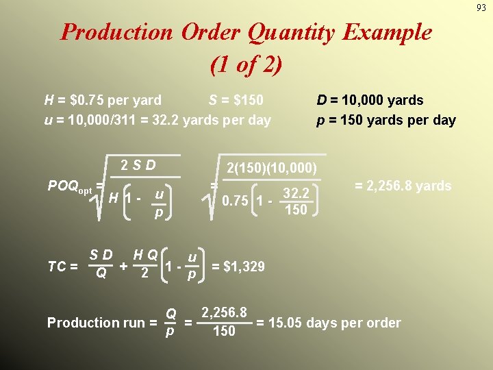
93 Production Order Quantity Example (1 of 2) H = $0. 75 per yard S = $150 u = 10, 000/311 = 32. 2 yards per day 2 SD POQopt = H 1 - u p SD HQ u TC = Q + 2 1 - p D = 10, 000 yards p = 150 yards per day 2(150)(10, 000) = 32. 2 0. 75 1 150 = 2, 256. 8 yards = $1, 329 2, 256. 8 Q Production run = = = 15. 05 days per order p 150

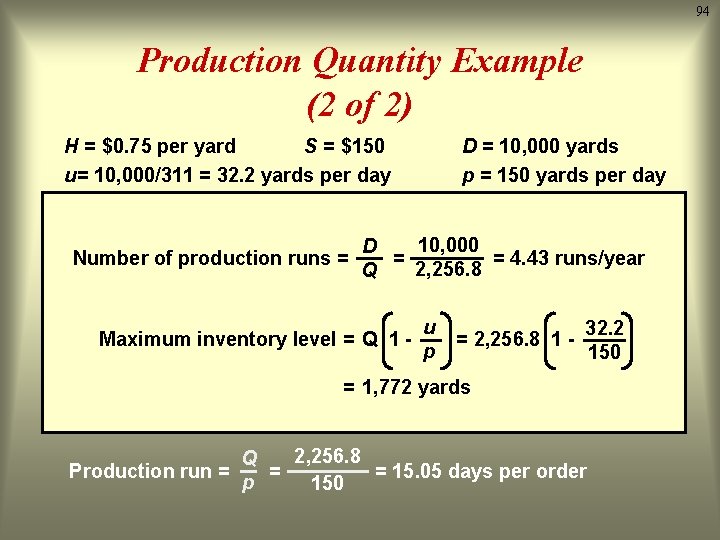
94 Production Quantity Example (2 of 2) H = $0. 75 per yard S = $150 u= 10, 000/311 = 32. 2 yards per day D = 10, 000 yards p = 150 yards per day 2 Co D 10, 000 2(150)(10, 000) D Number of production runs = = = 4. 43 runs/year 2, 256. 8 = 2, 256. 8 yards Q Qopt = = 32. 2 Cc 1 - d 0. 75 1 150 p u 32. 2 Maximum inventory level = Q 1 = 2, 256. 8 1 p 150 Co D Cc Q d = 1, 772 yards TC = Q + 2 1 - p = $1, 329 2, 256. 8 Q Production run = = = 15. 05 days per order p 150

95 Fixed-Order Quantity Models: Economic Order Quantity Model with Quantity Discounts

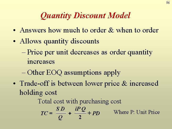
96 Quantity Discount Model • Answers how much to order & when to order • Allows quantity discounts – Price per unit decreases as order quantity increases – Other EOQ assumptions apply • Trade-off is between lower price & increased holding cost Total cost with purchasing cost SD i. P Q TC = + + PD Q 2 Where P: Unit Price

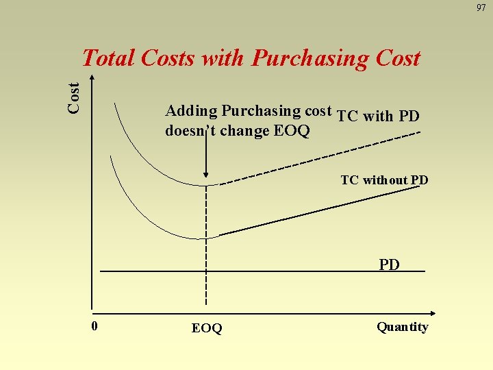
97 Cost Total Costs with Purchasing Cost Adding Purchasing cost TC with PD doesn’t change EOQ TC without PD PD 0 EOQ Quantity

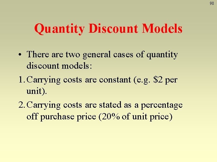
98 Quantity Discount Models • There are two general cases of quantity discount models: 1. Carrying costs are constant (e. g. $2 per unit). 2. Carrying costs are stated as a percentage off purchase price (20% of unit price)

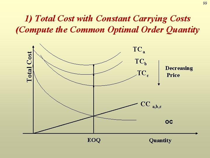
99 1) Total Cost with Constant Carrying Costs (Compute the Common Optimal Order Quantity Total Cost TCa TCb Decreasing Price TCc CC a, b, c OC EOQ Quantity

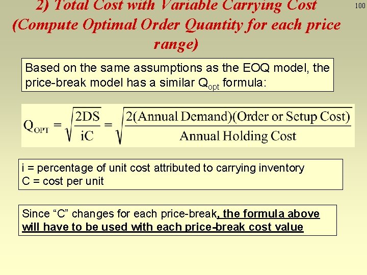
2) Total Cost with Variable Carrying Cost (Compute Optimal Order Quantity for each price range) Based on the same assumptions as the EOQ model, the price-break model has a similar Qopt formula: i = percentage of unit cost attributed to carrying inventory C = cost per unit Since “C” changes for each price-break, the formula above will have to be used with each price-break cost value 100

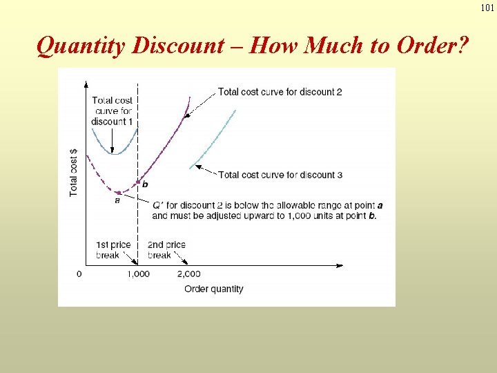
101 Quantity Discount – How Much to Order?

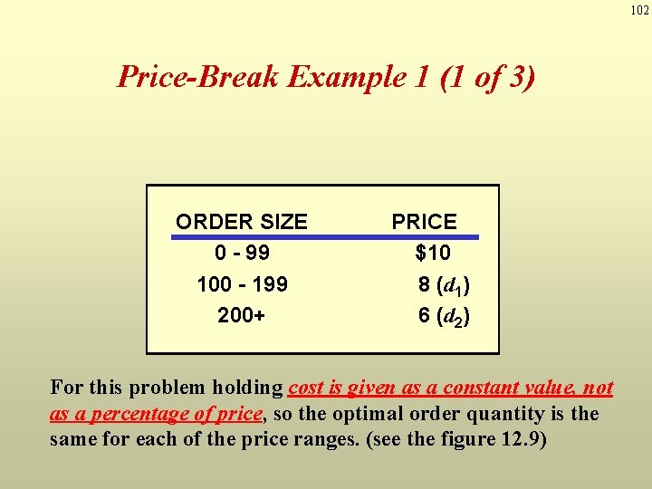
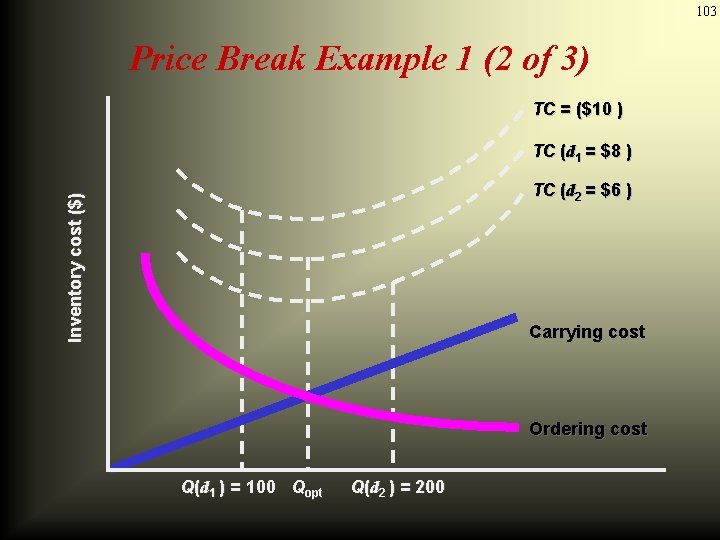
102 Price-Break Example 1 (1 of 3) ORDER SIZE 0 - 99 100 - 199 200+ PRICE $10 8 (d 1) 6 (d 2) For this problem holding cost is given as a constant value, not as a percentage of price, so the optimal order quantity is the same for each of the price ranges. (see the figure 12. 9)

103 Price Break Example 1 (2 of 3) TC = ($10 ) TC (d 1 = $8 ) Inventory cost ($) TC (d 2 = $6 ) Carrying cost Ordering cost Q(d 1 ) = 100 Qopt Q(d 2 ) = 200

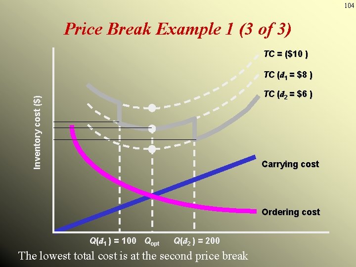
104 Price Break Example 1 (3 of 3) TC = ($10 ) TC (d 1 = $8 ) Inventory cost ($) TC (d 2 = $6 ) Carrying cost Ordering cost Q(d 1 ) = 100 Qopt Q(d 2 ) = 200 The lowest total cost is at the second price break

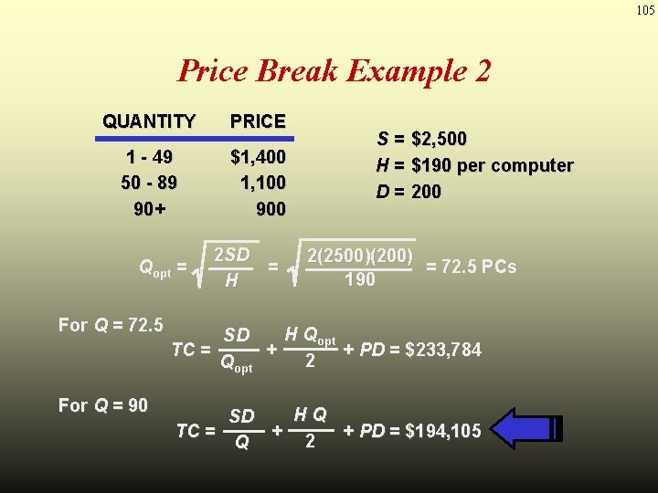
105 Price Break Example 2 QUANTITY PRICE 1 - 49 50 - 89 90+ $1, 400 1, 100 900 Qopt = For Q = 72. 5 For Q = 90 2 S D = H S= H= D= $2, 500 $190 per computer 200 2(2500)(200) = 72. 5 PCs 190 H Qopt SD TC = + + PD = $233, 784 2 Qopt HQ SD TC = + + PD = $194, 105 2 Q

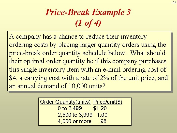
106 Price-Break Example 3 (1 of 4) A company has a chance to reduce their inventory ordering costs by placing larger quantity orders using the price-break order quantity schedule below. What should their optimal order quantity be if this company purchases this single inventory item with an e-mail ordering cost of $4, a carrying cost with a rate of 2% of the unit price, and an annual demand of 10, 000 units? Order Quantity(units) Price/unit($) 0 to 2, 499 $1. 20 2, 500 to 3, 999 1. 00 4, 000 or more. 98

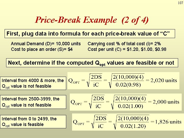
107 Price-Break Example (2 of 4) First, plug data into formula for each price-break value of “C” Annual Demand (D)= 10, 000 units Cost to place an order (S)= $4 Carrying cost % of total cost (i)= 2% Cost per unit (C) = $1. 20, $1. 00, $0. 98 Next, determine if the computed Qopt values are feasible or not Interval from 4000 & more, the Qopt value is not feasible Interval from 2500 -3999, the Qopt value is not feasible Interval from 0 to 2499, the Qopt value is feasible

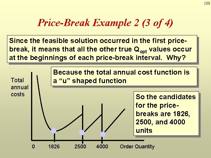
108 Price-Break Example 2 (3 of 4) Since the feasible solution occurred in the first pricebreak, it means that all the other true Qopt values occur at the beginnings of each price-break interval. Why? Because the total annual cost function is a “u” shaped function Total annual costs So the candidates for the pricebreaks are 1826, 2500, and 4000 units 0 1826 2500 4000 Order Quantity

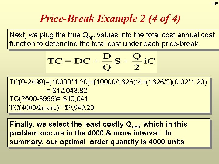
109 Price-Break Example 2 (4 of 4) Next, we plug the true Qopt values into the total cost annual cost function to determine the total cost under each price-break TC(0 -2499)=(10000*1. 20)+(10000/1826)*4+(1826/2)(0. 02*1. 20) = $12, 043. 82 TC(2500 -3999)= $10, 041 TC(4000&more)= $9, 949. 20 Finally, we select the least costly Qopt, which in this problem occurs in the 4000 & more interval. In summary, our optimal order quantity is 4000 units

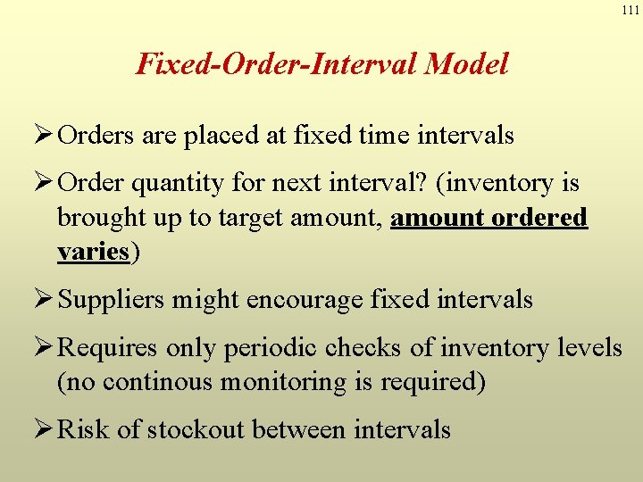
110 Multi-period Inventory Models: Fixed Time Period (Fixed-Order- Interval) Models

111 Fixed-Order-Interval Model Ø Orders are placed at fixed time intervals Ø Order quantity for next interval? (inventory is brought up to target amount, amount ordered varies) Ø Suppliers might encourage fixed intervals Ø Requires only periodic checks of inventory levels (no continous monitoring is required) Ø Risk of stockout between intervals

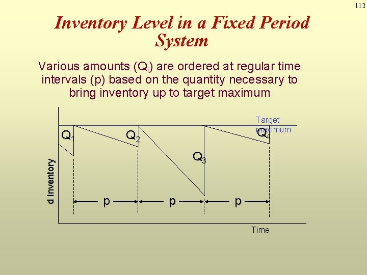
112 Inventory Level in a Fixed Period System Various amounts (Qi) are ordered at regular time intervals (p) based on the quantity necessary to bring inventory up to target maximum d Inventory Q 1 Target maximum Q 4 Q 2 Q 3 p p p Time

113 Fixed-Interval Benefits ØTight control of inventory items ØItems from same supplier may yield savings in: § Ordering § Packing § Shipping costs ØMay be practical when inventories cannot be closely monitored

114 Fixed-Interval Disadvantages Ø Requires a larger safety stock Ø Increases carrying cost Ø Costs of periodic reviews

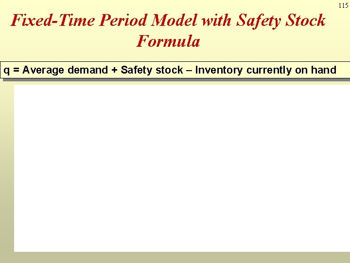
115 Fixed-Time Period Model with Safety Stock Formula q = Average demand + Safety stock – Inventory currently on hand

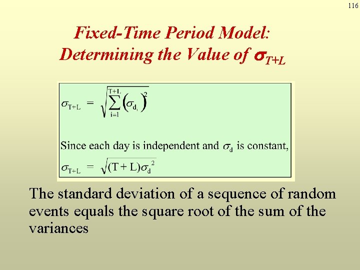
116 Fixed-Time Period Model: Determining the Value of s. T+L The standard deviation of a sequence of random events equals the square root of the sum of the variances

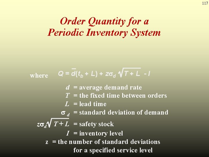
117 Order Quantity for a Periodic Inventory System where Q = d(tb + L) + z d d T L d T+L -I = average demand rate = the fixed time between orders = lead time = standard deviation of demand z d T + L = safety stock I = inventory level z = the number of standard deviations for a specified service level

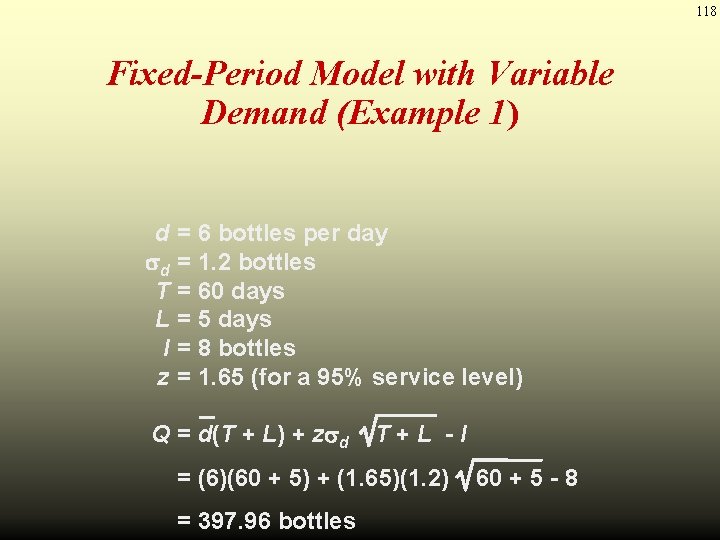
118 Fixed-Period Model with Variable Demand (Example 1) d d T L I z = 6 bottles per day = 1. 2 bottles = 60 days = 5 days = 8 bottles = 1. 65 (for a 95% service level) Q = d(T + L) + z d T+L -I = (6)(60 + 5) + (1. 65)(1. 2) = 397. 96 bottles 60 + 5 - 8

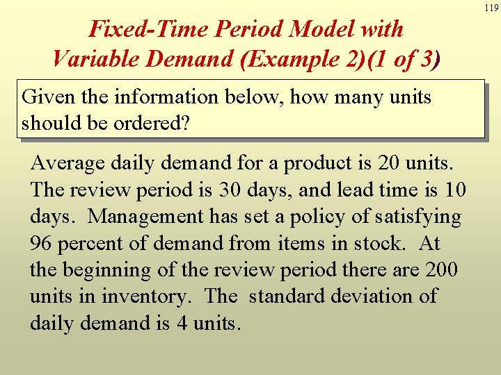
119 Fixed-Time Period Model with Variable Demand (Example 2)(1 of 3) Given the information below, how many units should be ordered? Average daily demand for a product is 20 units. The review period is 30 days, and lead time is 10 days. Management has set a policy of satisfying 96 percent of demand from items in stock. At the beginning of the review period there are 200 units in inventory. The standard deviation of daily demand is 4 units.

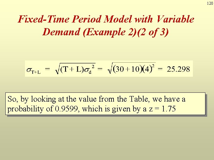
120 Fixed-Time Period Model with Variable Demand (Example 2)(2 of 3) So, by looking at the value from the Table, we have a probability of 0. 9599, which is given by a z = 1. 75

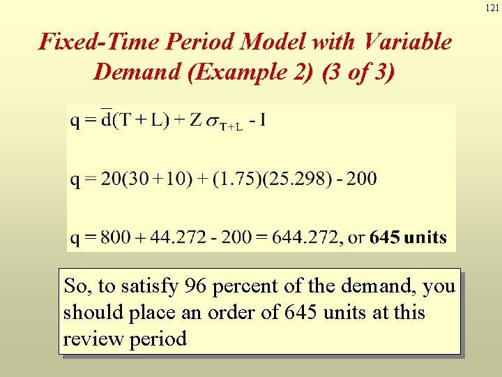
121 Fixed-Time Period Model with Variable Demand (Example 2) (3 of 3) So, to satisfy 96 percent of the demand, you should place an order of 645 units at this review period

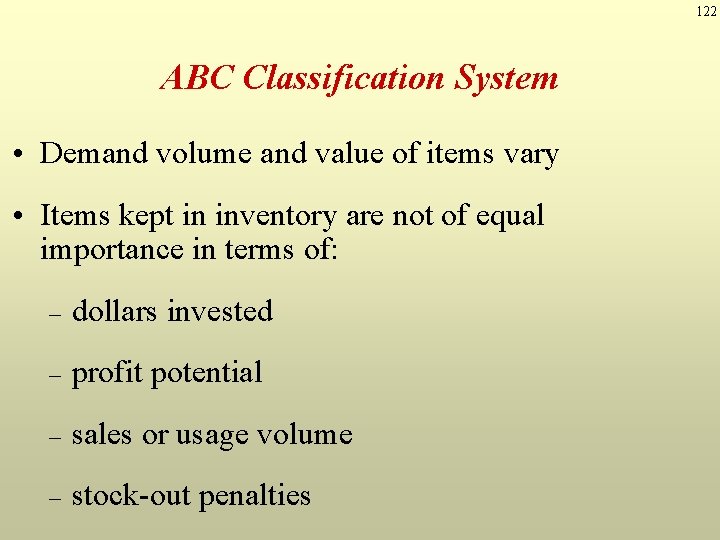
122 ABC Classification System • Demand volume and value of items vary • Items kept in inventory are not of equal importance in terms of: – dollars invested – profit potential – sales or usage volume – stock-out penalties

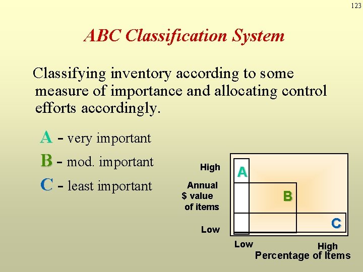
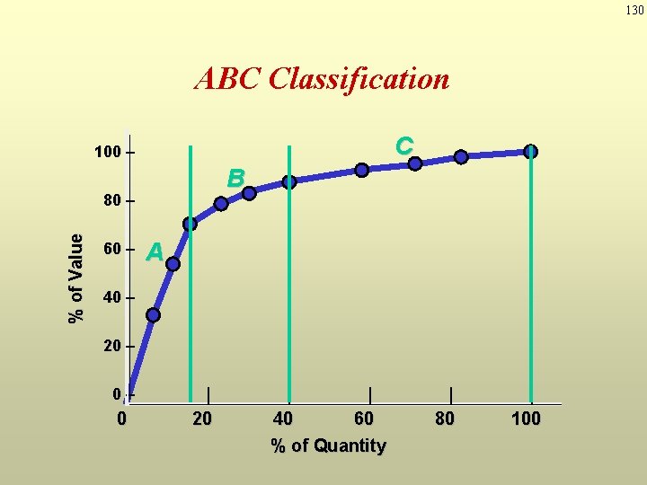
123 ABC Classification System Classifying inventory according to some measure of importance and allocating control efforts accordingly. A - very important B - mod. important C - least important High Annual $ value of items A B C Low High Percentage of Items

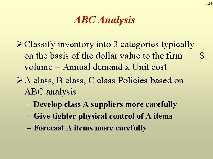
124 ABC Analysis Ø Classify inventory into 3 categories typically on the basis of the dollar value to the firm $ volume = Annual demand x Unit cost Ø A class, B class, C class Policies based on ABC analysis – Develop class A suppliers more carefully – Give tighter physical control of A items – Forecast A items more carefully

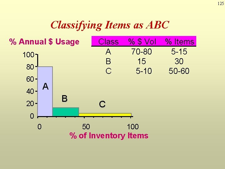
125 Classifying Items as ABC Class A B C % Annual $ Usage 100 80 60 % $ Vol 70 -80 15 5 -10 A 40 B 20 C 0 0 50 100 % of Inventory Items % Items 5 -15 30 50 -60

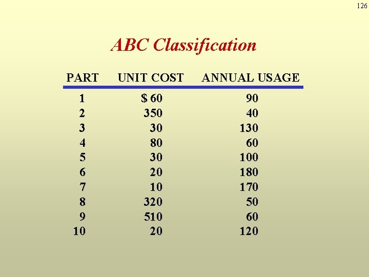
126 ABC Classification PART UNIT COST ANNUAL USAGE 1 2 3 4 5 6 7 8 9 10 $ 60 350 30 80 30 20 10 320 510 20 90 40 130 60 100 180 170 50 60 120

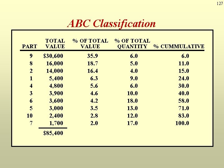
127 ABC Classification PART 9 8 2 1 4 3 6 5 10 7 TOTAL % OF TOTAL PART UNIT ANNUAL USAGE VALUECOSTQUANTITY % CUMMULATIVE $30, 600 1 16, 000 2 14, 000 3 5, 400 4 4, 800 5 3, 900 3, 600 6 3, 000 7 2, 400 8 1, 700 9 $85, 400 10 35. 9 $ 60 18. 7 350 16. 4 30 6. 3 5. 680 4. 630 4. 220 3. 510 2. 8 320 2. 0 510 20 6. 0 5. 0 4. 0 9. 0 6. 0 10. 0 18. 0 13. 0 12. 0 17. 0 90 40 130 60 100 180 170 50 60 120 6. 0 11. 0 15. 0 24. 0 30. 0 40. 0 58. 0 71. 0 83. 0 100. 0

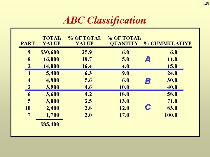
128 ABC Classification PART 9 8 2 1 4 3 6 5 10 7 TOTAL % OF TOTAL PART UNIT ANNUAL USAGE VALUECOSTQUANTITY % CUMMULATIVE $30, 600 1 16, 000 2 14, 000 3 5, 400 4 4, 800 5 3, 900 3, 600 6 3, 000 7 2, 400 8 1, 700 9 $85, 400 10 35. 9 $ 60 18. 7 350 16. 4 30 6. 3 5. 680 4. 630 4. 220 3. 510 2. 8 320 2. 0 510 20 6. 0 5. 0 4. 0 9. 0 6. 0 10. 0 18. 0 13. 0 12. 0 17. 0 90 A 40 130 60 B 100 180 170 C 50 60 120 6. 0 11. 0 15. 0 24. 0 30. 0 40. 0 58. 0 71. 0 83. 0 100. 0

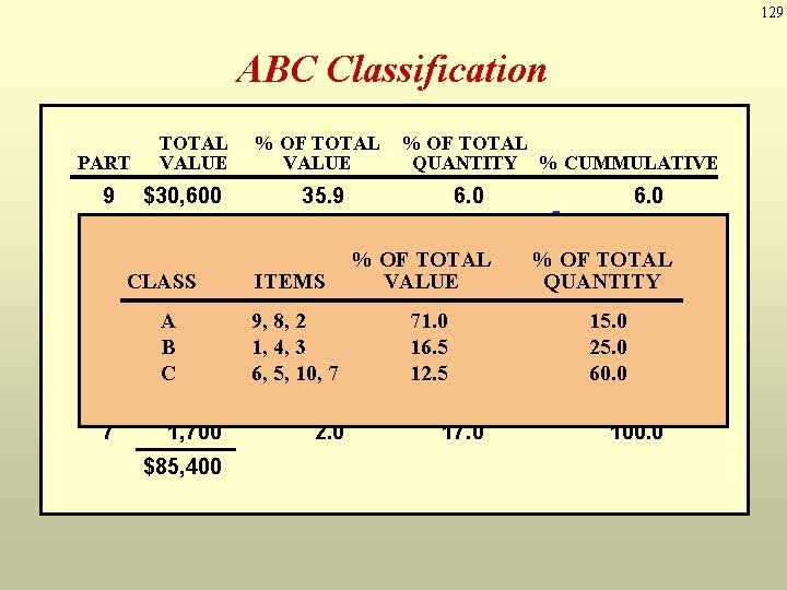
129 ABC Classification PART TOTAL % OF TOTAL PART UNIT ANNUAL USAGE VALUECOSTQUANTITY % CUMMULATIVE 9 $30, 600 1 8 16, 000 2 2 14, 000 3 1 CLASS 5, 400 4 4 4, 800 A 3, 900 5 3 B 3, 600 6 6 C 3, 000 5 7 10 2, 400 8 7 1, 700 9 $85, 400 10 35. 9 6. 0 $ 60 18. 7 5. 0 350 16. 4 % OF TOTAL 4. 0 30 6. 3 ITEMS VALUE 9. 0 5. 680 6. 0 9, 8, 2 4. 630 71. 010. 0 1, 4, 3 4. 220 16. 518. 0 6, 5, 10, 3. 5 7 12. 513. 0 10 2. 8 12. 0 320 2. 0 17. 0 510 20 6. 0 90 11. 0 A 40 15. 0 % OF TOTAL 130 24. 0 QUANTITY 60 B 15. 030. 0 100 40. 0 180 25. 058. 0 60. 071. 0 170 C 83. 0 50 100. 0 60 120

130 ABC Classification C 100 – B % of Value 80 – 60 – A 40 – 20 – 0 | 20 | | 40 60 % of Quantity | 80 | 100

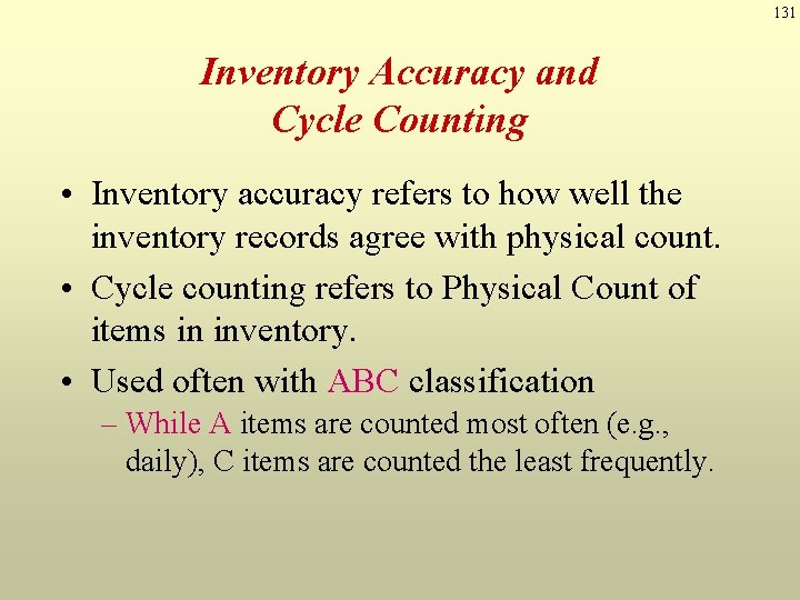
131 Inventory Accuracy and Cycle Counting • Inventory accuracy refers to how well the inventory records agree with physical count. • Cycle counting refers to Physical Count of items in inventory. • Used often with ABC classification – While A items are counted most often (e. g. , daily), C items are counted the least frequently.

132 Last Words Inventories have certain functions. But too much inventory - Tends to hide problems - Costly to maintain So it is desired • Reduce lot sizes • Reduce safety stocks