1 Inventory Management and Control 2 AMAZON com

1 Inventory Management and Control

2 AMAZON. com • Jeff Bezos, in 1995, started AMAZON. com as a “virtual” retailer – no inventory, no warehouses, no overhead; just a bunch of computers. • Growth forced AMAZON. com to excel in inventory management! • AMAZON is now a worldwide leader in warehouse management and automation.

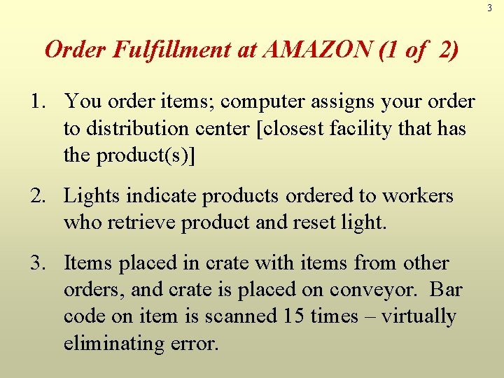
3 Order Fulfillment at AMAZON (1 of 2) 1. You order items; computer assigns your order to distribution center [closest facility that has the product(s)] 2. Lights indicate products ordered to workers who retrieve product and reset light. 3. Items placed in crate with items from other orders, and crate is placed on conveyor. Bar code on item is scanned 15 times – virtually eliminating error.

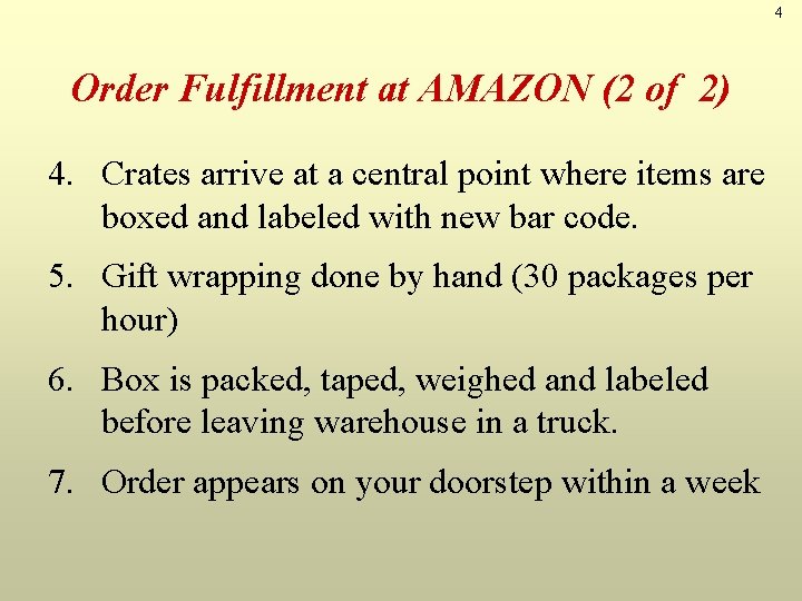
4 Order Fulfillment at AMAZON (2 of 2) 4. Crates arrive at a central point where items are boxed and labeled with new bar code. 5. Gift wrapping done by hand (30 packages per hour) 6. Box is packed, taped, weighed and labeled before leaving warehouse in a truck. 7. Order appears on your doorstep within a week

5 Inventory Defined • Inventory is the stock of any item or resource held to meet future demand can include: raw materials, finished products, component parts, supplies, and work-in-process

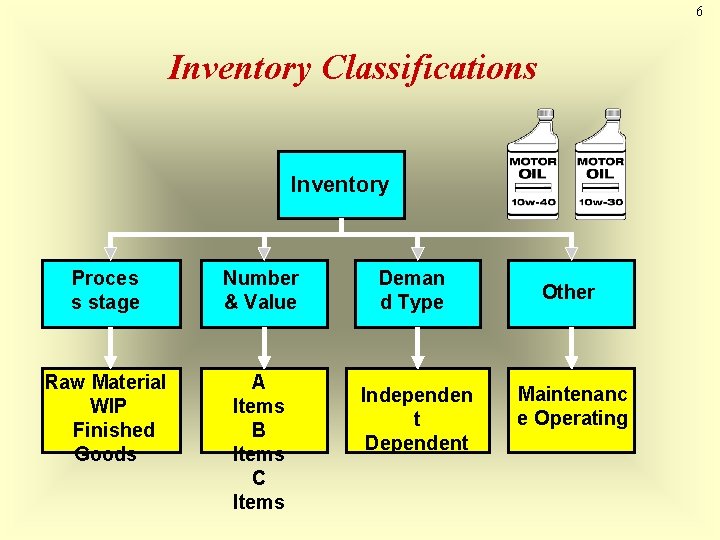
6 Inventory Classifications Inventory Proces s stage Number & Value Raw Material WIP Finished Goods A Items B Items C Items Deman d Type Independen t Dependent Other Maintenanc e Operating

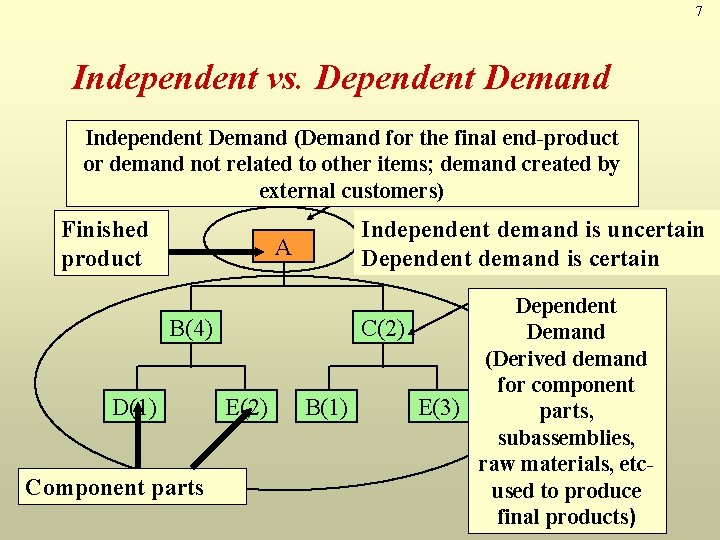
7 Independent vs. Dependent Demand Independent Demand (Demand for the final end-product or demand not related to other items; demand created by external customers) Finished product A B(4) D(1) Component parts E(1) E(2) Independent demand is uncertain Dependent demand is certain Dependent C(2) Demand (Derived demand for component B(1) E(3) parts, subassemblies, raw materials, etcused to produce final products)

8 Inventory Models • Independent demand – finished goods, items that are ready to be sold – E. g. a computer • Dependent demand – components of finished products – E. g. parts that make up the computer

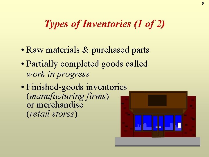
9 Types of Inventories (1 of 2) • Raw materials & purchased parts • Partially completed goods called work in progress • Finished-goods inventories (manufacturing firms) or merchandise (retail stores)

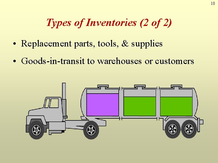
10 Types of Inventories (2 of 2) • Replacement parts, tools, & supplies • Goods-in-transit to warehouses or customers

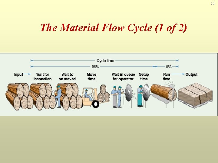
11 The Material Flow Cycle (1 of 2)

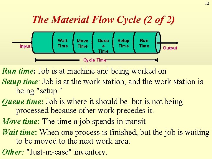
12 The Material Flow Cycle (2 of 2) Input Wait Time Move Time Queu e Time Setup Time Run Time Output Cycle Time Run time: Job is at machine and being worked on Setup time: Job is at the work station, and the work station is being "setup. " Queue time: Job is where it should be, but is not being processed because other work precedes it. Move time: The time a job spends in transit Wait time: When one process is finished, but the job is waiting to be moved to the next work area. Other: "Just-in-case" inventory.

13 Performance Measures • Inventory turnover (the ratio of annual cost of goods sold to average inventory investment) • Days of inventory on hand (expected number of days of sales that can be supplied from existing inventory)

14 Functions of Inventory (1 of 2) 1. To “decouple” or separate various parts of the production process, ie. to maintain independence of operations 2. To meet unexpected demand & to provide high levels of customer service 3. To smooth production requirements by meeting seasonal or cyclical variations in demand 4. To protect against stock-outs

15 Functions of Inventory (2 of 2) 5. To provide a safeguard for variation in raw material delivery time 6. To provide a stock of goods that will provide a “selection” for customers 7. To take advantage of economic purchase-order size 8. To take advantage of quantity discounts 9. To hedge against price increases

16 Disadvantages of Inventory • Higher costs – Item cost (if purchased) – Ordering (or setup) cost – Holding (or carrying) cost • Difficult to control • Hides production problems • May decrease flexibility

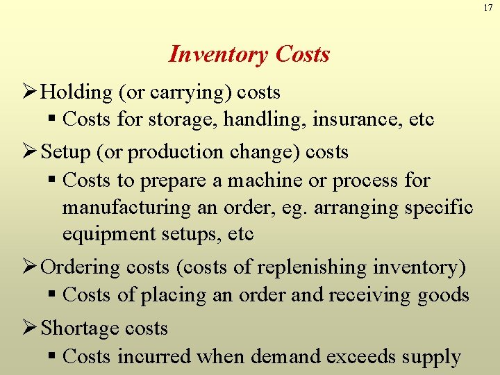
17 Inventory Costs Ø Holding (or carrying) costs § Costs for storage, handling, insurance, etc Ø Setup (or production change) costs § Costs to prepare a machine or process for manufacturing an order, eg. arranging specific equipment setups, etc Ø Ordering costs (costs of replenishing inventory) § Costs of placing an order and receiving goods Ø Shortage costs § Costs incurred when demand exceeds supply

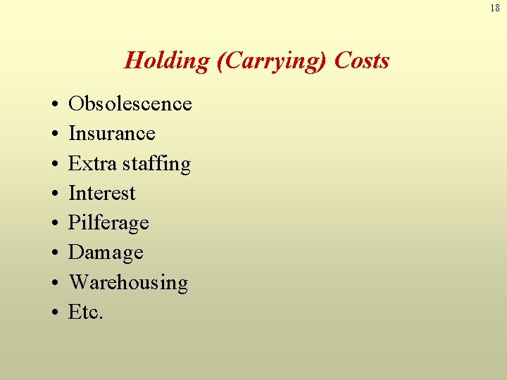
18 Holding (Carrying) Costs • • Obsolescence Insurance Extra staffing Interest Pilferage Damage Warehousing Etc.

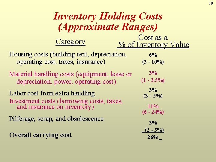
19 Inventory Holding Costs (Approximate Ranges) Category Cost as a % of Inventory Value Housing costs (building rent, depreciation, operating cost, taxes, insurance) 6% (3 - 10%) Material handling costs (equipment, lease or depreciation, power, operating cost) 3% (1 - 3. 5%) Labor cost from extra handling Investment costs (borrowing costs, taxes, and insurance on inventory) Pilferage, scrap, and obsolescence Overall carrying cost 3% (3 - 5%) 11% (6 - 24%) 3% (2 - 5%) 26%

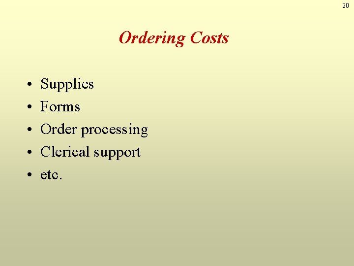
20 Ordering Costs • • • Supplies Forms Order processing Clerical support etc.

21 Setup Costs • • Clean-up costs Re-tooling costs Adjustment costs etc.

22 Shortage Costs • Backordering cost • Cost of lost sales

23 Inventory Control System Defined Ø An inventory system is the set of policies and controls that monitor levels of inventory and determine what levels should be maintained, when stock should be replenished and how large orders should be Ø Answers questions as: § When to order? § How much to order?

24 Objective of Inventory Control To achieve satisfactory levels of customer service while keeping inventory costs within reasonable bounds ØLevel of customer service ØCosts of ordering and carrying inventory

25 Requirements of an Effective Inventory Management ØA system to keep track of inventory ØA reliable forecast of demand ØKnowledge of lead times ØReasonable estimates of § Holding costs § Ordering costs § Shortage costs ØA classification system

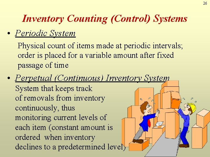
26 Inventory Counting (Control) Systems • Periodic System Physical count of items made at periodic intervals; order is placed for a variable amount after fixed passage of time • Perpetual (Continuous) Inventory System that keeps track of removals from inventory continuously, thus monitoring current levels of each item (constant amount is ordered when inventory declines to a predetermined level)

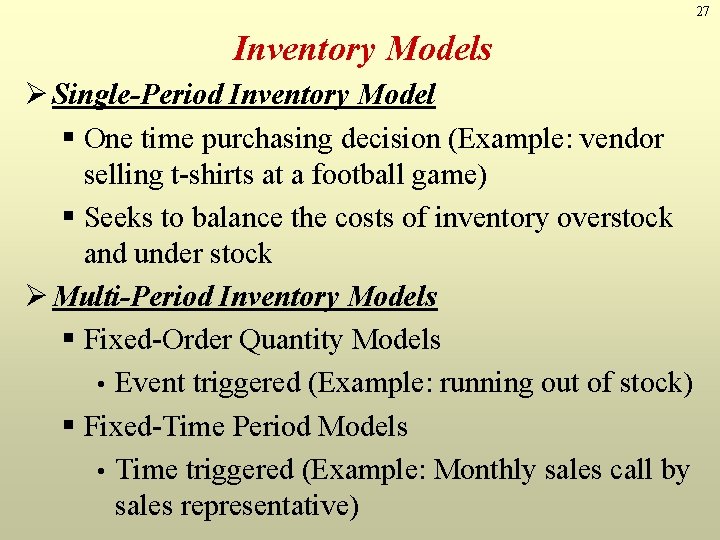
27 Inventory Models Ø Single-Period Inventory Model § One time purchasing decision (Example: vendor selling t-shirts at a football game) § Seeks to balance the costs of inventory overstock and under stock Ø Multi-Period Inventory Models § Fixed-Order Quantity Models • Event triggered (Example: running out of stock) § Fixed-Time Period Models • Time triggered (Example: Monthly sales call by sales representative)

28 Single-Period Inventory Model

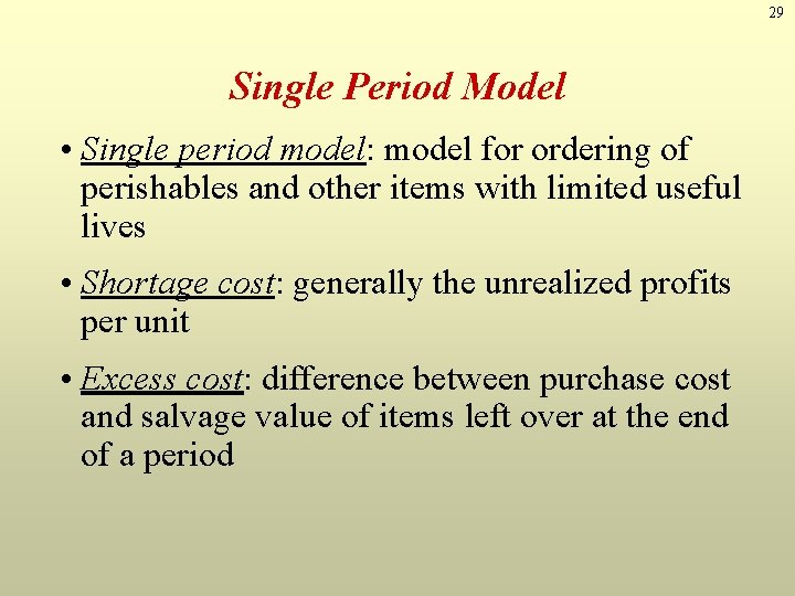
29 Single Period Model • Single period model: model for ordering of perishables and other items with limited useful lives • Shortage cost: generally the unrealized profits per unit • Excess cost: difference between purchase cost and salvage value of items left over at the end of a period

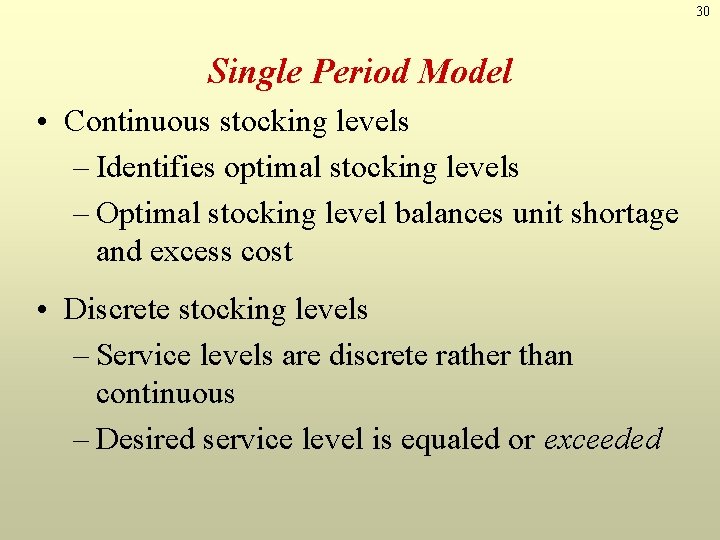
30 Single Period Model • Continuous stocking levels – Identifies optimal stocking levels – Optimal stocking level balances unit shortage and excess cost • Discrete stocking levels – Service levels are discrete rather than continuous – Desired service level is equaled or exceeded

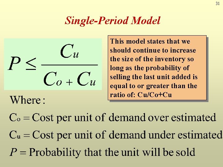
31 Single-Period Model This model states that we should continue to increase the size of the inventory so long as the probability of selling the last unit added is equal to or greater than the ratio of: Cu/Co+Cu

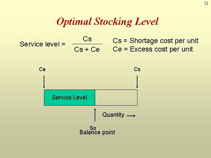
32 Optimal Stocking Level Service level = Cs Cs + Ce Cs = Shortage cost per unit Ce = Excess cost per unit Ce Cs Service Level Quantity So Balance point

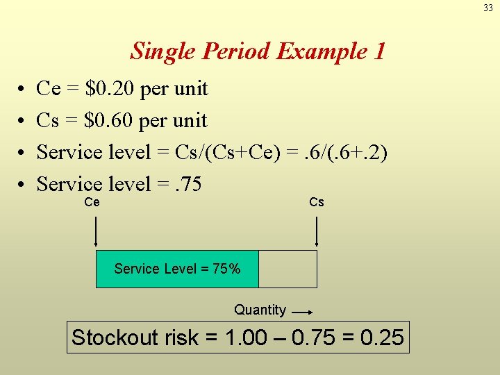
33 Single Period Example 1 • • Ce = $0. 20 per unit Cs = $0. 60 per unit Service level = Cs/(Cs+Ce) =. 6/(. 6+. 2) Service level =. 75 Ce Cs Service Level = 75% Quantity Stockout risk = 1. 00 – 0. 75 = 0. 25

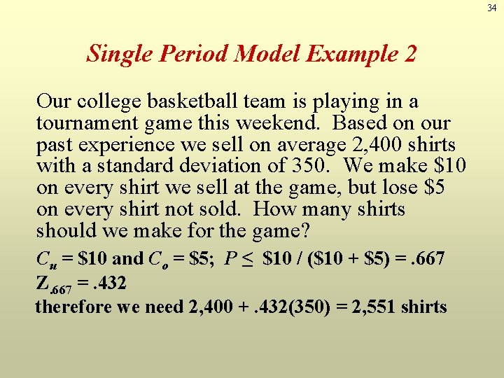
34 Single Period Model Example 2 Our college basketball team is playing in a tournament game this weekend. Based on our past experience we sell on average 2, 400 shirts with a standard deviation of 350. We make $10 on every shirt we sell at the game, but lose $5 on every shirt not sold. How many shirts should we make for the game? Cu = $10 and Co = $5; P ≤ $10 / ($10 + $5) =. 667 Z. 667 =. 432 therefore we need 2, 400 +. 432(350) = 2, 551 shirts

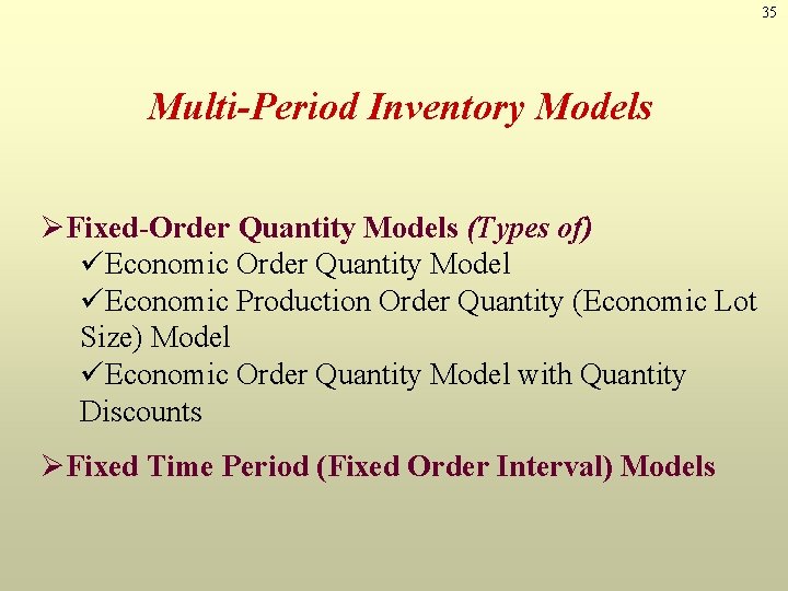
35 Multi-Period Inventory Models ØFixed-Order Quantity Models (Types of) üEconomic Order Quantity Model üEconomic Production Order Quantity (Economic Lot Size) Model üEconomic Order Quantity Model with Quantity Discounts ØFixed Time Period (Fixed Order Interval) Models

36 Fixed Order Quantity Models: Economic Order Quantity Model

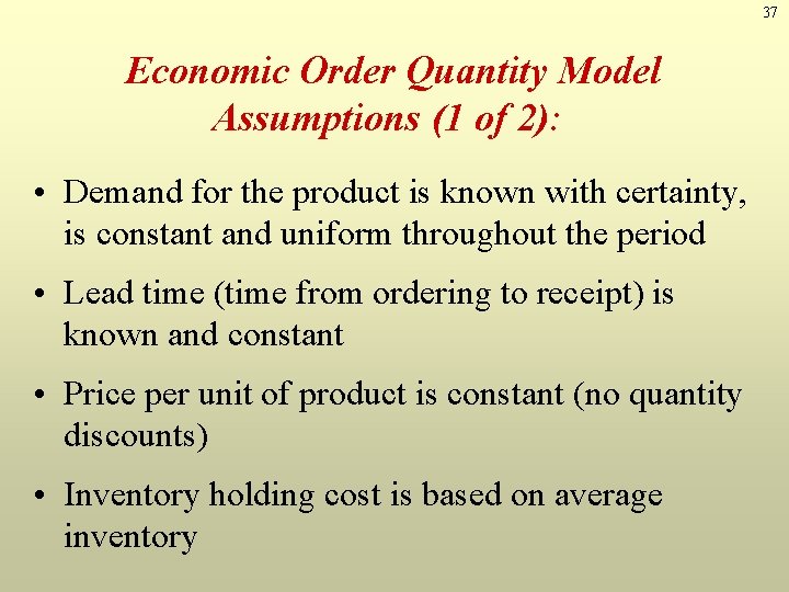
37 Economic Order Quantity Model Assumptions (1 of 2): • Demand for the product is known with certainty, is constant and uniform throughout the period • Lead time (time from ordering to receipt) is known and constant • Price per unit of product is constant (no quantity discounts) • Inventory holding cost is based on average inventory

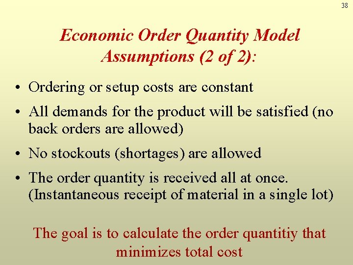
38 Economic Order Quantity Model Assumptions (2 of 2): • Ordering or setup costs are constant • All demands for the product will be satisfied (no back orders are allowed) • No stockouts (shortages) are allowed • The order quantity is received all at once. (Instantaneous receipt of material in a single lot) The goal is to calculate the order quantitiy that minimizes total cost

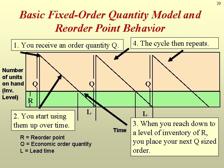
39 Basic Fixed-Order Quantity Model and Reorder Point Behavior 1. You receive an order quantity Q. Number of units on hand (Inv. Level) Q Q 4. The cycle then repeats. Q R 2. You start using them up over time. L R = Reorder point Q = Economic order quantity L = Lead time Time L 3. When you reach down to a level of inventory of R, you place your next Q sized order.

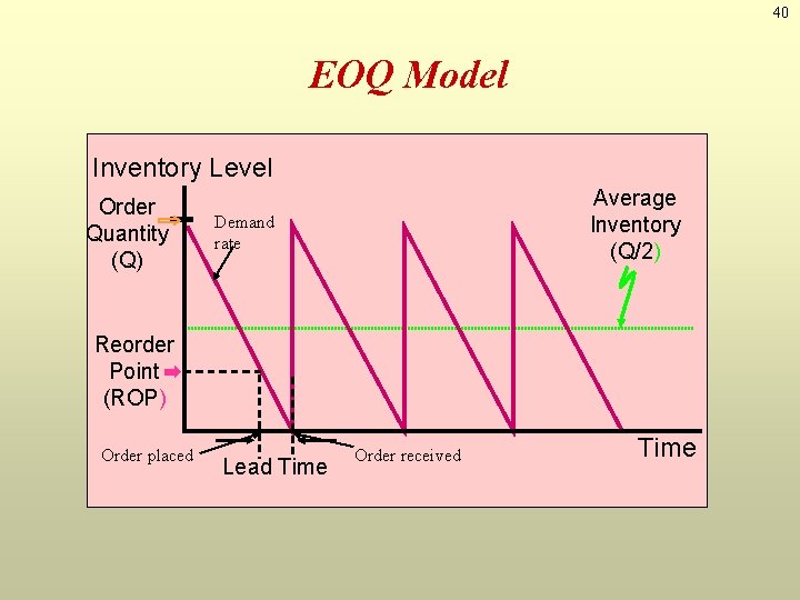
40 EOQ Model Inventory Level Order Quantity (Q) Average Inventory (Q/2) Demand rate Reorder Point (ROP) Order placed Lead Time Order received Time

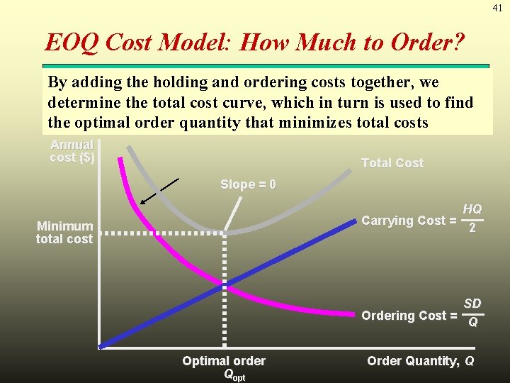
41 EOQ Cost Model: How Much to Order? By adding the holding and ordering costs together, we determine the total cost curve, which in turn is used to find the optimal order quantity that minimizes total costs Annual cost ($) Total Cost Slope = 0 HQ Carrying Cost = 2 Minimum total cost SD Ordering Cost = Q Optimal order Qopt Order Quantity, Q

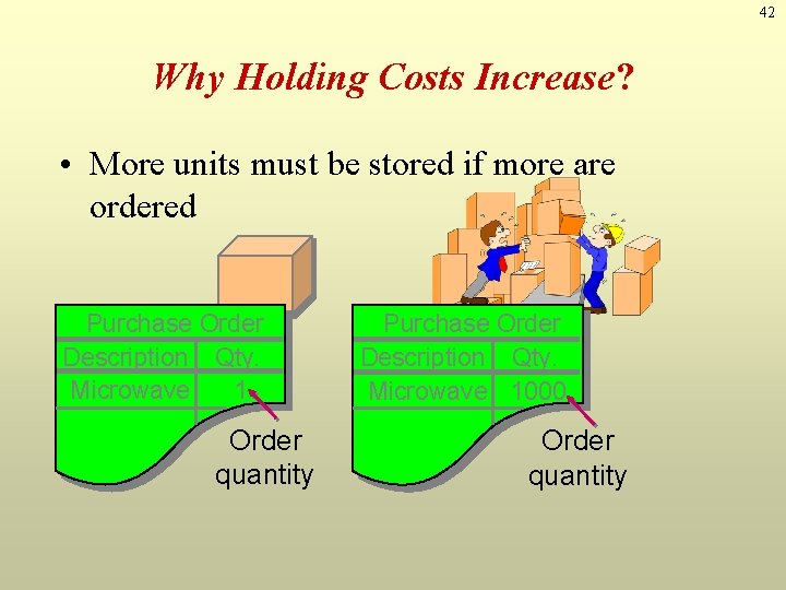
42 Why Holding Costs Increase? • More units must be stored if more are ordered Purchase Order Description Qty. Microwave 1 Order quantity Purchase Order Description Qty. Microwave 1000 Order quantity

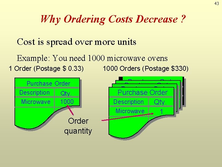
43 Why Ordering Costs Decrease ? Cost is spread over more units Example: You need 1000 microwave ovens 1 Order (Postage $ 0. 33) 1000 Orders (Postage $330) Purchase Order Description Qty. Microwave 1000 Purchase. Order Description Qty. Purchase Description Qty. 1 Microwave Description Qty. Microwave 11 Microwave 1 Order quantity

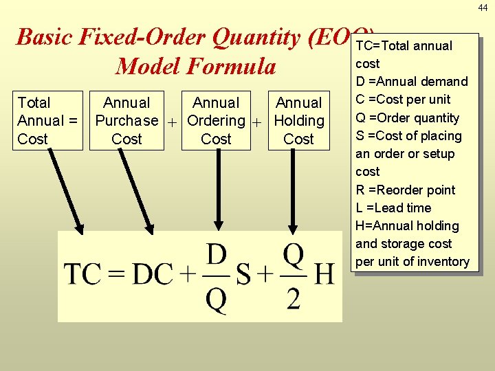
44 Basic Fixed-Order Quantity (EOQ) TC=Total annual cost Model Formula D =Annual demand Total Annual = Cost Annual Purchase + Ordering + Holding Cost C =Cost per unit Q =Order quantity S =Cost of placing an order or setup cost R =Reorder point L =Lead time H=Annual holding and storage cost per unit of inventory

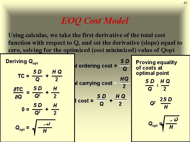
45 EOQ Cost Model Using calculus, we take the first derivative of the total cost function with respect to Q, and set the derivative (slope) equal to zero, solving for the optimized (cost minimized) value of Qopt Deriving Qopt SD Annual ordering cost = Q SD HQ TC = + HQ Q 2 Annual carrying cost = 2 SD H TC = 2 + Q 2 SD HQ Q Total cost = + Q 2 SD H 0= + Q 2 2 Qopt = 2 SD H Proving equality of costs at optimal point SD HQ = Q 2 2 S D Q 2 = H 2 SD Qopt = H

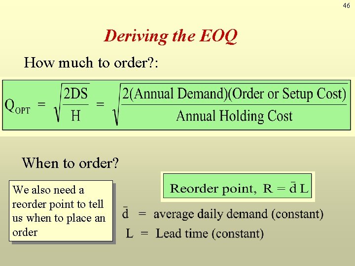
46 Deriving the EOQ How much to order? : When to order? We also need a reorder point to tell us when to place an order

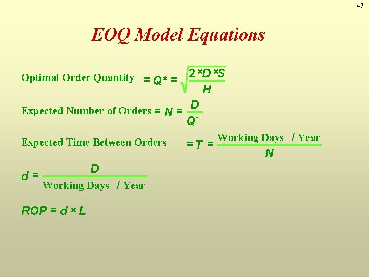
47 EOQ Model Equations 2 ×D ×S H D Expected Number of Orders = N = Q* Optimal Order Quantity = Q* = Expected Time Between Orders d= D Working Days / Year ROP = d × L =T = Working Days / Year N

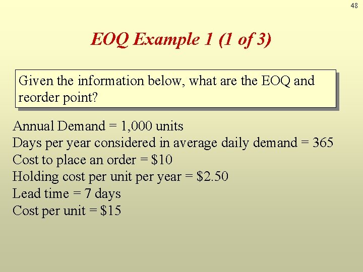
48 EOQ Example 1 (1 of 3) Given the information below, what are the EOQ and reorder point? Annual Demand = 1, 000 units Days per year considered in average daily demand = 365 Cost to place an order = $10 Holding cost per unit per year = $2. 50 Lead time = 7 days Cost per unit = $15

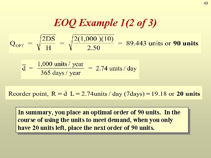
49 EOQ Example 1(2 of 3) In summary, you place an optimal order of 90 units. In the course of using the units to meet demand, when you only have 20 units left, place the next order of 90 units.

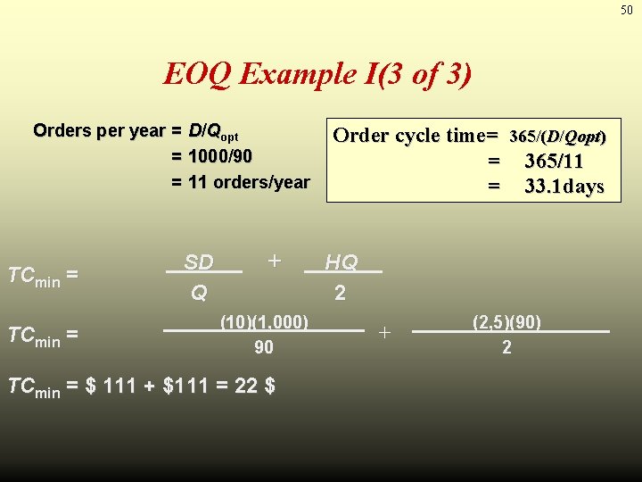
50 EOQ Example I(3 of 3) Orders per year = D/Qopt = 1000/90 = 11 orders/year TCmin = SD Q + (10)(1, 000) 90 TCmin = $ 111 + $111 = 22 $ Order cycle time= 365/(D/Qopt) = 365/11 = 33. 1 days HQ 2 + (2, 5)(90) 2

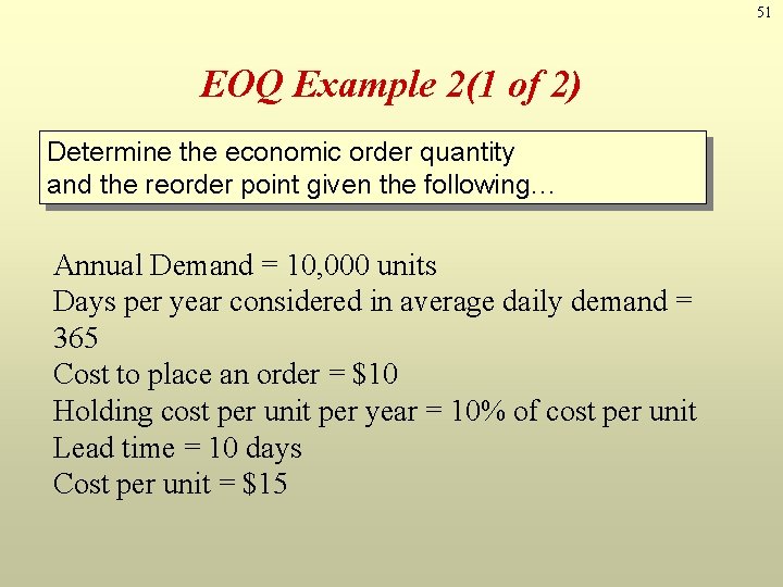
51 EOQ Example 2(1 of 2) Determine the economic order quantity and the reorder point given the following… Annual Demand = 10, 000 units Days per year considered in average daily demand = 365 Cost to place an order = $10 Holding cost per unit per year = 10% of cost per unit Lead time = 10 days Cost per unit = $15

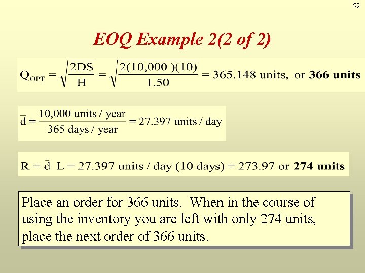
52 EOQ Example 2(2 of 2) Place an order for 366 units. When in the course of using the inventory you are left with only 274 units, place the next order of 366 units.

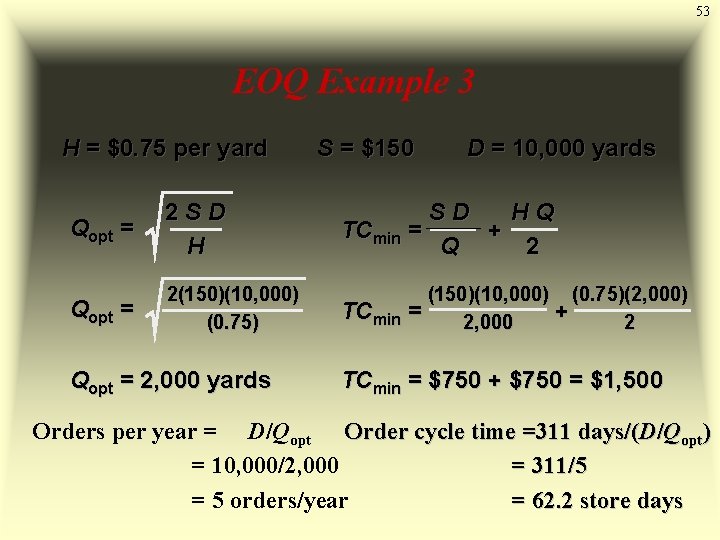
53 EOQ Example 3 H = $0. 75 per yard Qopt = 2 SD H Qopt = 2(150)(10, 000) (0. 75) Qopt = 2, 000 yards S = $150 D = 10, 000 yards SD HQ TCmin = + Q 2 TCmin (150)(10, 000) (0. 75)(2, 000) = + 2, 000 2 TCmin = $750 + $750 = $1, 500 Orders per year = D/Qopt Order cycle time =311 days/(D/Qopt) = 10, 000/2, 000 = 311/5 = 5 orders/year = 62. 2 store days

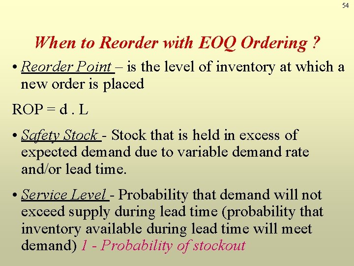
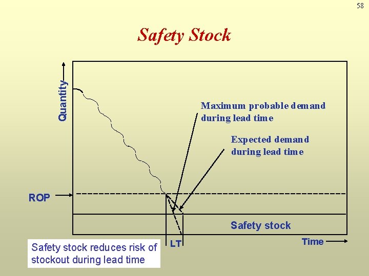
54 When to Reorder with EOQ Ordering ? • Reorder Point – is the level of inventory at which a new order is placed ROP = d. L • Safety Stock - Stock that is held in excess of expected demand due to variable demand rate and/or lead time. • Service Level - Probability that demand will not exceed supply during lead time (probability that inventory available during lead time will meet demand) 1 - Probability of stockout

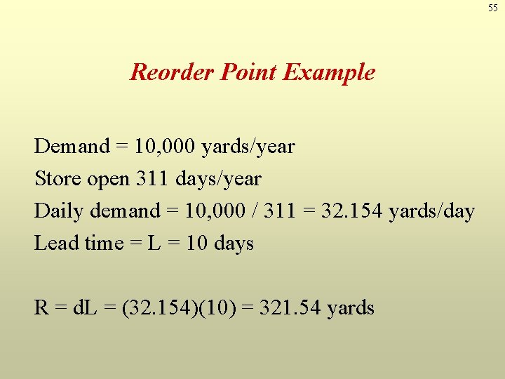
55 Reorder Point Example Demand = 10, 000 yards/year Store open 311 days/year Daily demand = 10, 000 / 311 = 32. 154 yards/day Lead time = L = 10 days R = d. L = (32. 154)(10) = 321. 54 yards

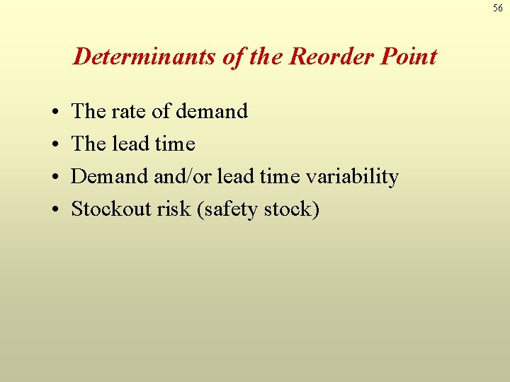
56 Determinants of the Reorder Point • • The rate of demand The lead time Demand and/or lead time variability Stockout risk (safety stock)

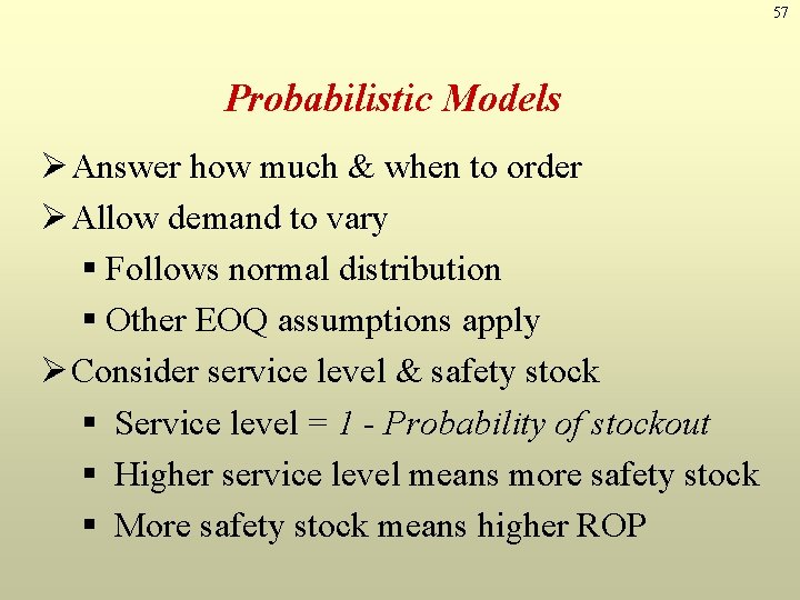
57 Probabilistic Models Ø Answer how much & when to order Ø Allow demand to vary § Follows normal distribution § Other EOQ assumptions apply Ø Consider service level & safety stock § Service level = 1 - Probability of stockout § Higher service level means more safety stock § More safety stock means higher ROP

58 Quantity Safety Stock Maximum probable demand during lead time Expected demand during lead time ROP Safety stock reduces risk of stockout during lead time LT Time

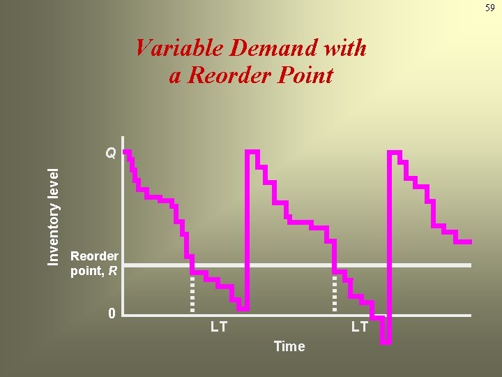
59 Variable Demand with a Reorder Point Inventory level Q Reorder point, R 0 LT LT Time

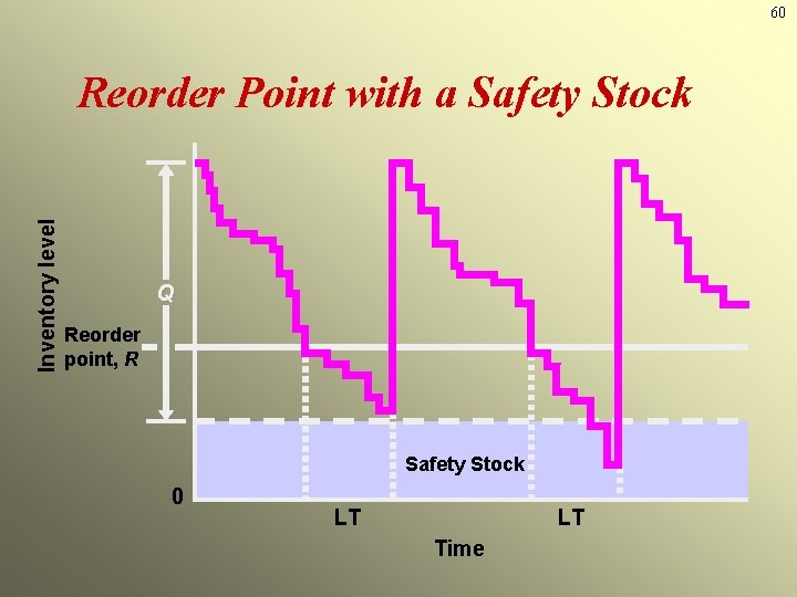
60 Inventory level Reorder Point with a Safety Stock Q Reorder point, R Safety Stock 0 LT LT Time

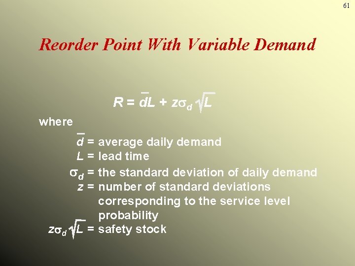
61 Reorder Point With Variable Demand R = d. L + z d L where d = average daily demand L = lead time d = the standard deviation of daily demand z = number of standard deviations corresponding to the service level probability z d L = safety stock

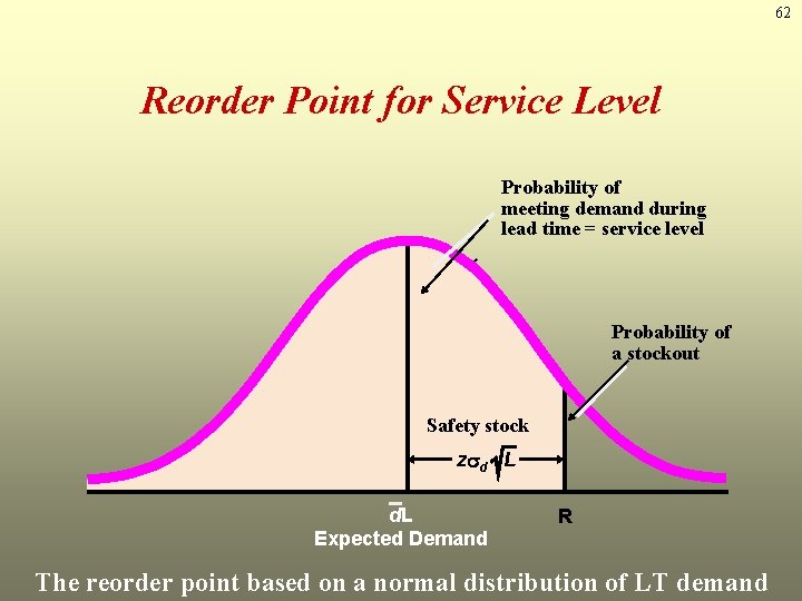
62 Reorder Point for Service Level Probability of meeting demand during lead time = service level Probability of a stockout Safety stock z d L d. L Expected Demand R The reorder point based on a normal distribution of LT demand

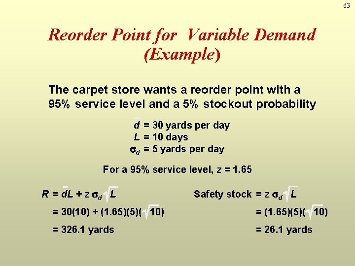
63 Reorder Point for Variable Demand (Example) The carpet store wants a reorder point with a 95% service level and a 5% stockout probability d = 30 yards per day L = 10 days d = 5 yards per day For a 95% service level, z = 1. 65 R = d. L + z d L Safety stock = z d L = 30(10) + (1. 65)(5)( 10) = 326. 1 yards = 26. 1 yards

64 Fixed Order Quantity Models: -Noninstantaneous Receipt. Production Order Quantity (Economic Lot Size) Model

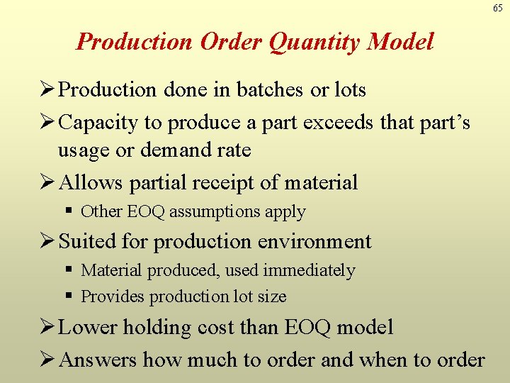
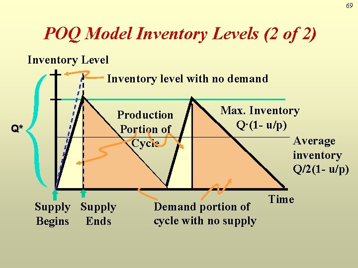
65 Production Order Quantity Model Ø Production done in batches or lots Ø Capacity to produce a part exceeds that part’s usage or demand rate Ø Allows partial receipt of material § Other EOQ assumptions apply Ø Suited for production environment § Material produced, used immediately § Provides production lot size Ø Lower holding cost than EOQ model Ø Answers how much to order and when to order

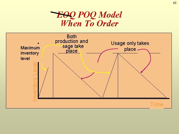
66 EOQ POQ Model When To Order Inventory Level Maximum inventory level Both production and usage take place Usage only takes place Time

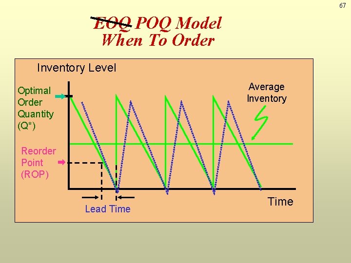
67 EOQ POQ Model When To Order Inventory Level Average Inventory Optimal Order Quantity (Q*) Reorder Point (ROP) Lead Time

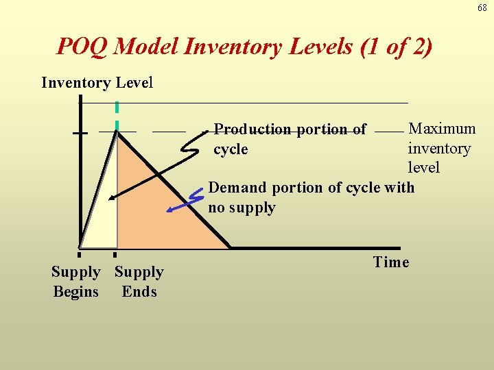
68 POQ Model Inventory Levels (1 of 2) Inventory Level Maximum inventory level Demand portion of cycle with no supply Production portion of cycle Supply Begins Ends Time

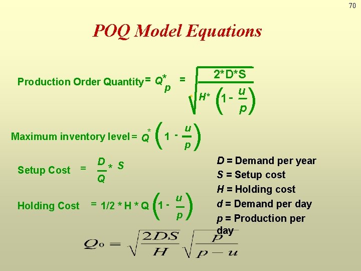
69 POQ Model Inventory Levels (2 of 2) Inventory Level Inventory level with no demand Production Portion of Cycle Q* Supply Begins Ends Max. Inventory Q·(1 - u/p) Average inventory Q/2(1 - u/p) Demand portion of cycle with no supply Time

70 POQ Model Equations Production Order Quantity = Q* = p Maximum inventory level = Q* Setup Cost = Holding Cost D Q 2*D*S u H* 1 p ( ) 1 - u p * S ( ) = 1/2 * H * Q 1 - u p D = Demand per year S = Setup cost H = Holding cost d = Demand per day p = Production per day

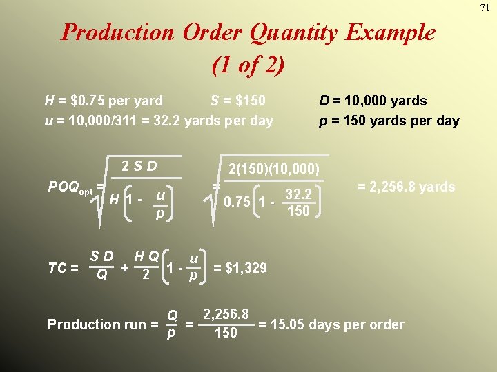
71 Production Order Quantity Example (1 of 2) H = $0. 75 per yard S = $150 u = 10, 000/311 = 32. 2 yards per day 2 SD POQopt = H 1 - u p SD HQ u TC = Q + 2 1 - p D = 10, 000 yards p = 150 yards per day 2(150)(10, 000) = 32. 2 0. 75 1 150 = 2, 256. 8 yards = $1, 329 2, 256. 8 Q Production run = = = 15. 05 days per order p 150

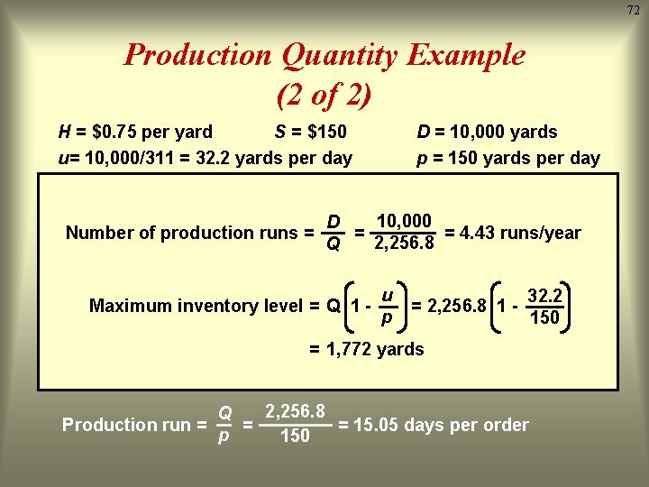
72 Production Quantity Example (2 of 2) H = $0. 75 per yard S = $150 u= 10, 000/311 = 32. 2 yards per day D = 10, 000 yards p = 150 yards per day 2 Co D 10, 000 2(150)(10, 000) D Number of production runs = = = 4. 43 runs/year 2, 256. 8 = 2, 256. 8 yards Q Qopt = = 32. 2 Cc 1 - d 0. 75 1 150 p u 32. 2 Maximum inventory level = Q 1 = 2, 256. 8 1 p 150 Co D Cc Q d = 1, 772 yards TC = Q + 2 1 - p = $1, 329 2, 256. 8 Q Production run = = = 15. 05 days per order p 150

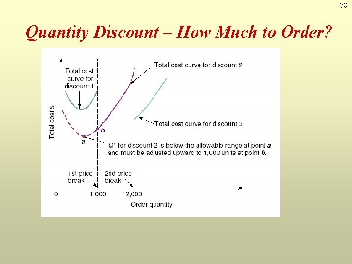
73 Fixed-Order Quantity Models: Economic Order Quantity Model with Quantity Discounts

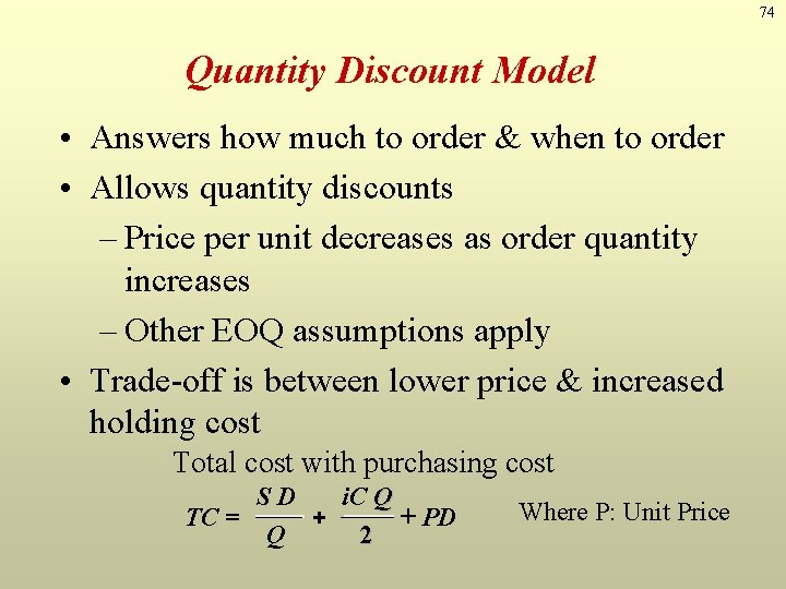
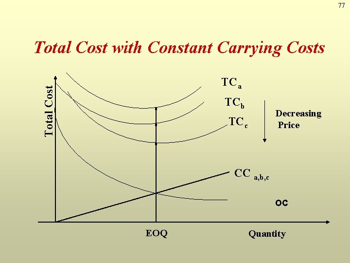
74 Quantity Discount Model • Answers how much to order & when to order • Allows quantity discounts – Price per unit decreases as order quantity increases – Other EOQ assumptions apply • Trade-off is between lower price & increased holding cost Total cost with purchasing cost SD i. C Q TC = + + PD Q 2 Where P: Unit Price

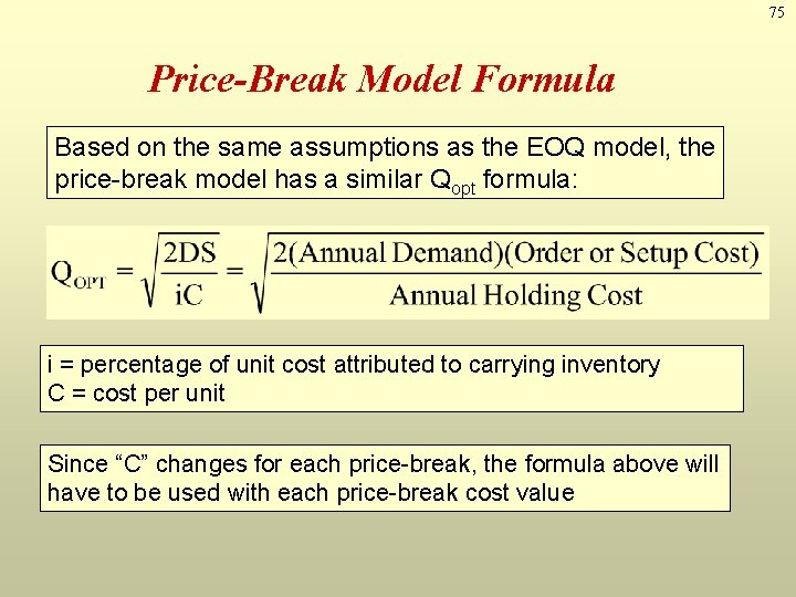
75 Price-Break Model Formula Based on the same assumptions as the EOQ model, the price-break model has a similar Qopt formula: i = percentage of unit cost attributed to carrying inventory C = cost per unit Since “C” changes for each price-break, the formula above will have to be used with each price-break cost value

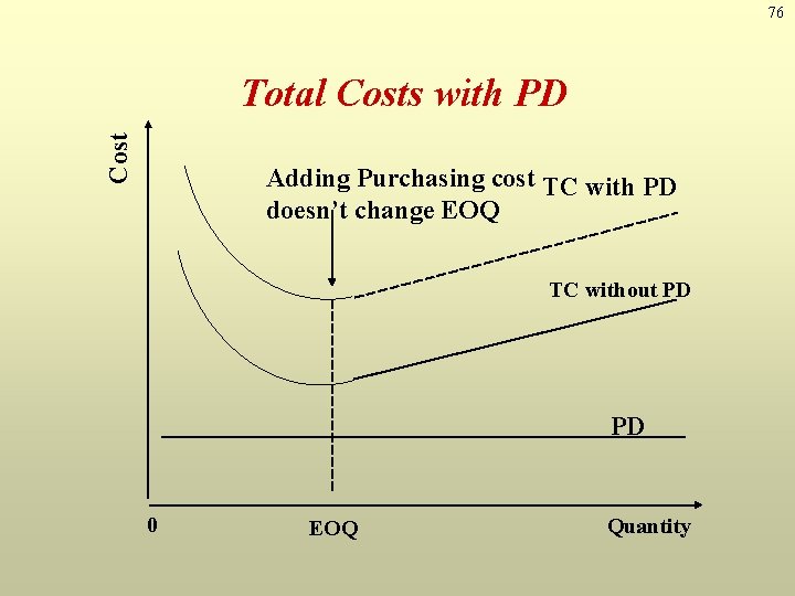
76 Cost Total Costs with PD Adding Purchasing cost TC with PD doesn’t change EOQ TC without PD PD 0 EOQ Quantity

77 Total Cost with Constant Carrying Costs Total Cost TCa TCb Decreasing Price TCc CC a, b, c OC EOQ Quantity

78 Quantity Discount – How Much to Order?

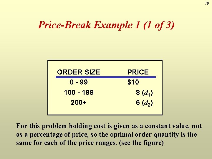
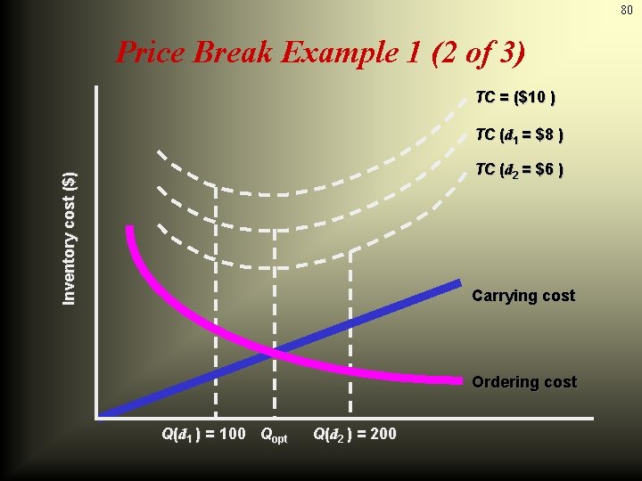
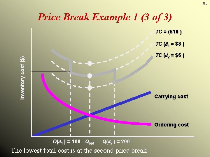
79 Price-Break Example 1 (1 of 3) ORDER SIZE 0 - 99 100 - 199 200+ PRICE $10 8 (d 1) 6 (d 2) For this problem holding cost is given as a constant value, not as a percentage of price, so the optimal order quantity is the same for each of the price ranges. (see the figure)

80 Price Break Example 1 (2 of 3) TC = ($10 ) TC (d 1 = $8 ) Inventory cost ($) TC (d 2 = $6 ) Carrying cost Ordering cost Q(d 1 ) = 100 Qopt Q(d 2 ) = 200

81 Price Break Example 1 (3 of 3) TC = ($10 ) TC (d 1 = $8 ) Inventory cost ($) TC (d 2 = $6 ) Carrying cost Ordering cost Q(d 1 ) = 100 Qopt Q(d 2 ) = 200 The lowest total cost is at the second price break

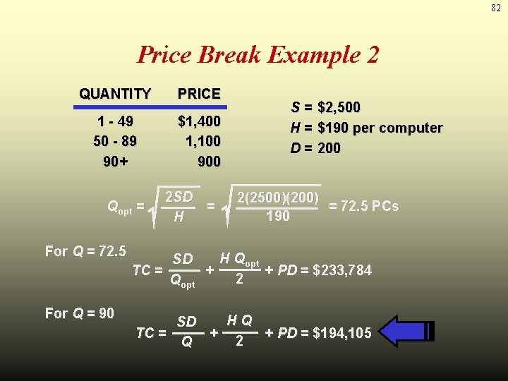
82 Price Break Example 2 QUANTITY PRICE 1 - 49 50 - 89 90+ $1, 400 1, 100 900 Qopt = For Q = 72. 5 For Q = 90 2 S D = H S= H= D= $2, 500 $190 per computer 200 2(2500)(200) = 72. 5 PCs 190 H Qopt SD TC = + + PD = $233, 784 2 Qopt HQ SD TC = + + PD = $194, 105 2 Q

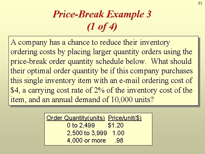
83 Price-Break Example 3 (1 of 4) A company has a chance to reduce their inventory ordering costs by placing larger quantity orders using the price-break order quantity schedule below. What should their optimal order quantity be if this company purchases this single inventory item with an e-mail ordering cost of $4, a carrying cost rate of 2% of the inventory cost of the item, and an annual demand of 10, 000 units? Order Quantity(units) Price/unit($) 0 to 2, 499 $1. 20 2, 500 to 3, 999 1. 00 4, 000 or more. 98

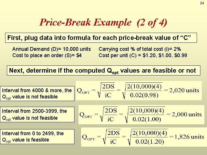
84 Price-Break Example (2 of 4) First, plug data into formula for each price-break value of “C” Annual Demand (D)= 10, 000 units Cost to place an order (S)= $4 Carrying cost % of total cost (i)= 2% Cost per unit (C) = $1. 20, $1. 00, $0. 98 Next, determine if the computed Qopt values are feasible or not Interval from 4000 & more, the Qopt value is not feasible Interval from 2500 -3999, the Qopt value is not feasible Interval from 0 to 2499, the Qopt value is feasible

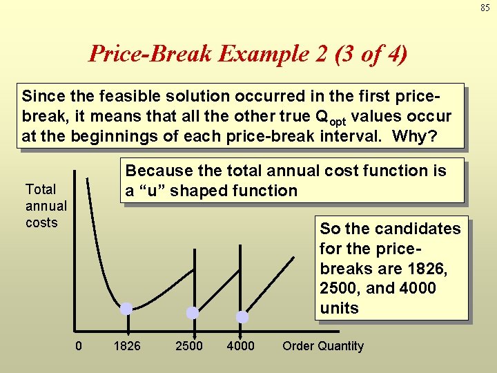
85 Price-Break Example 2 (3 of 4) Since the feasible solution occurred in the first pricebreak, it means that all the other true Qopt values occur at the beginnings of each price-break interval. Why? Because the total annual cost function is a “u” shaped function Total annual costs So the candidates for the pricebreaks are 1826, 2500, and 4000 units 0 1826 2500 4000 Order Quantity

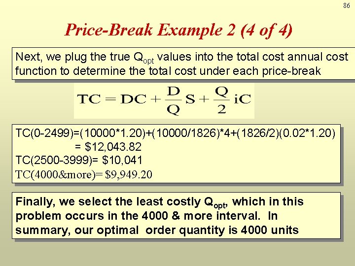
86 Price-Break Example 2 (4 of 4) Next, we plug the true Qopt values into the total cost annual cost function to determine the total cost under each price-break TC(0 -2499)=(10000*1. 20)+(10000/1826)*4+(1826/2)(0. 02*1. 20) = $12, 043. 82 TC(2500 -3999)= $10, 041 TC(4000&more)= $9, 949. 20 Finally, we select the least costly Qopt, which in this problem occurs in the 4000 & more interval. In summary, our optimal order quantity is 4000 units

87 Multi-period Inventory Models: Fixed Time Period (Fixed-Order- Interval) Models

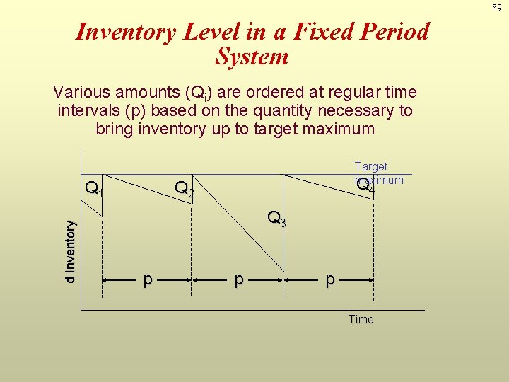
88 Fixed-Order-Interval Model Ø Orders are placed at fixed time intervals Ø Order quantity for next interval? (inventory is brought up to target amount, amount ordered varies) Ø Suppliers might encourage fixed intervals Ø Requires only periodic checks of inventory levels (no continous monitoring is required) Ø Risk of stockout between intervals

89 Inventory Level in a Fixed Period System Various amounts (Qi) are ordered at regular time intervals (p) based on the quantity necessary to bring inventory up to target maximum d Inventory Q 1 Target maximum Q 4 Q 2 Q 3 p p p Time

90 Fixed-Interval Benefits ØTight control of inventory items ØItems from same supplier may yield savings in: § Ordering § Packing § Shipping costs ØMay be practical when inventories cannot be closely monitored

91 Fixed-Interval Disadvantages Ø Requires a larger safety stock Ø Increases carrying cost Ø Costs of periodic reviews

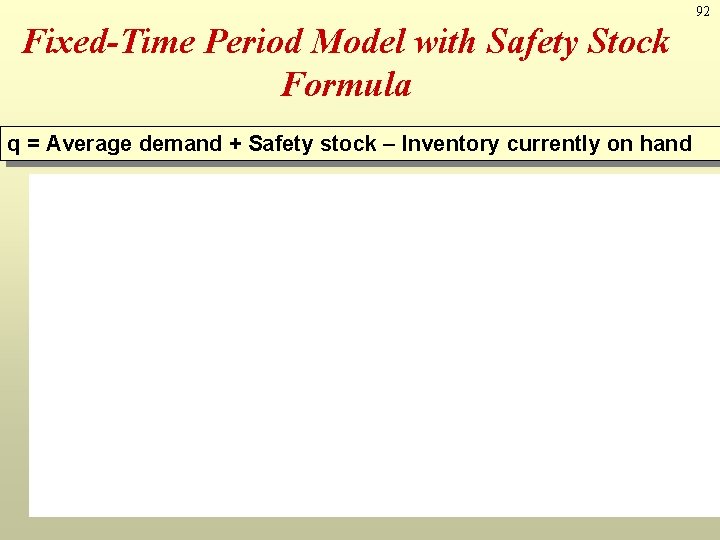
92 Fixed-Time Period Model with Safety Stock Formula q = Average demand + Safety stock – Inventory currently on hand

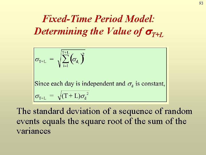
93 Fixed-Time Period Model: Determining the Value of s. T+L The standard deviation of a sequence of random events equals the square root of the sum of the variances

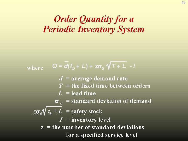
94 Order Quantity for a Periodic Inventory System where Q = d(tb + L) + z d d T L d T+L -I = average demand rate = the fixed time between orders = lead time = standard deviation of demand z d tb + L = safety stock I = inventory level z = the number of standard deviations for a specified service level

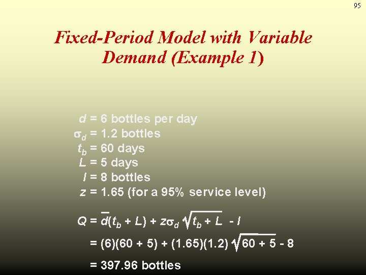
95 Fixed-Period Model with Variable Demand (Example 1) d d tb L I z = 6 bottles per day = 1. 2 bottles = 60 days = 5 days = 8 bottles = 1. 65 (for a 95% service level) Q = d(tb + L) + z d tb + L - I = (6)(60 + 5) + (1. 65)(1. 2) = 397. 96 bottles 60 + 5 - 8

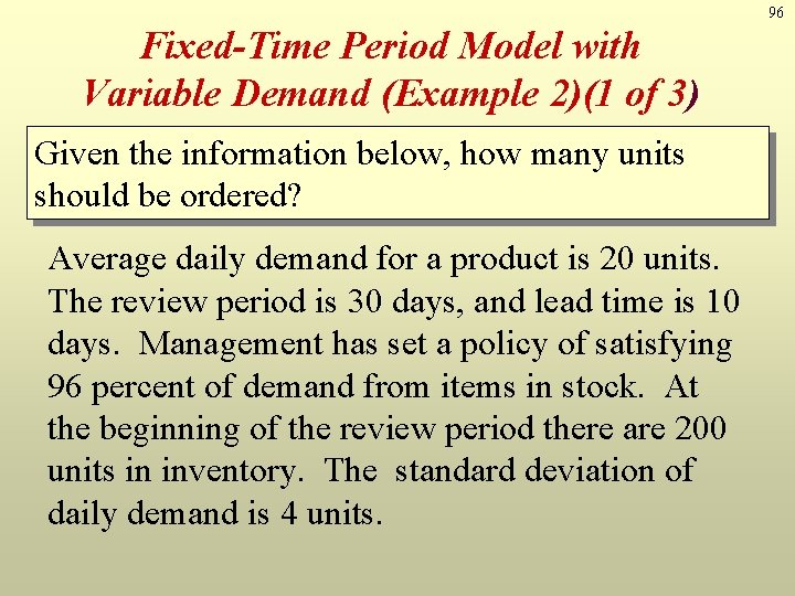
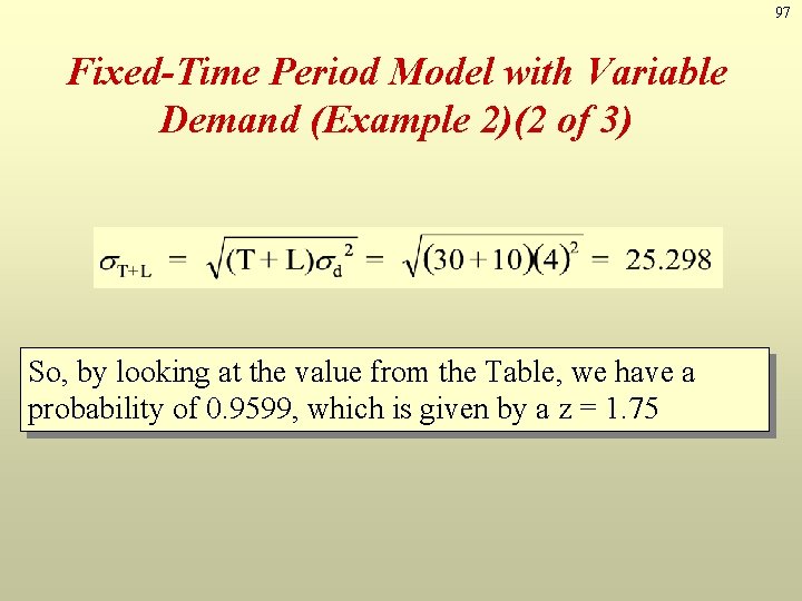
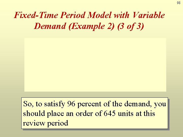
96 Fixed-Time Period Model with Variable Demand (Example 2)(1 of 3) Given the information below, how many units should be ordered? Average daily demand for a product is 20 units. The review period is 30 days, and lead time is 10 days. Management has set a policy of satisfying 96 percent of demand from items in stock. At the beginning of the review period there are 200 units in inventory. The standard deviation of daily demand is 4 units.

97 Fixed-Time Period Model with Variable Demand (Example 2)(2 of 3) So, by looking at the value from the Table, we have a probability of 0. 9599, which is given by a z = 1. 75

98 Fixed-Time Period Model with Variable Demand (Example 2) (3 of 3) So, to satisfy 96 percent of the demand, you should place an order of 645 units at this review period

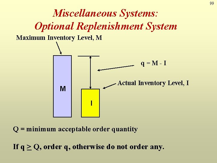
99 Miscellaneous Systems: Optional Replenishment System Maximum Inventory Level, M q=M-I Actual Inventory Level, I M I Q = minimum acceptable order quantity If q > Q, order q, otherwise do not order any.

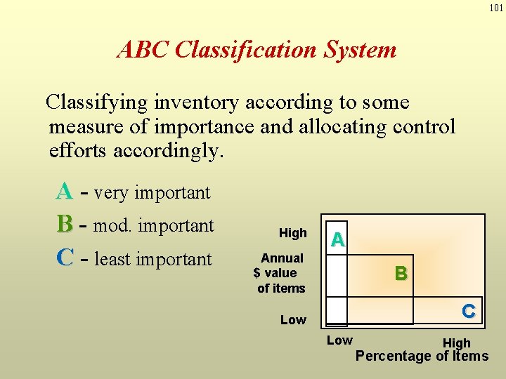
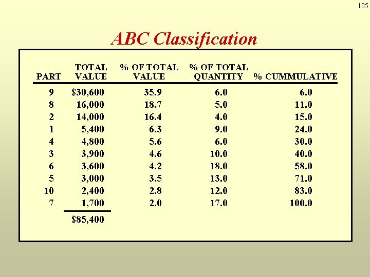
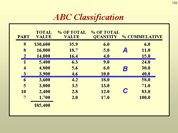
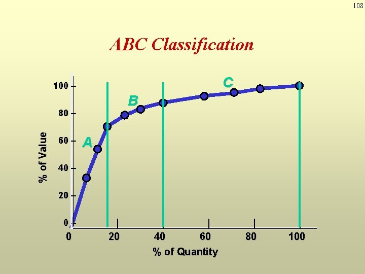
100 ABC Classification System • Demand volume and value of items vary • Items kept in inventory are not of equal importance in terms of: – dollars invested – profit potential – sales or usage volume – stock-out penalties

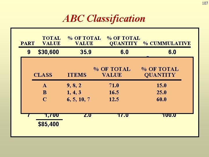
101 ABC Classification System Classifying inventory according to some measure of importance and allocating control efforts accordingly. A - very important B - mod. important C - least important High Annual $ value of items A B C Low High Percentage of Items

102 ABC Analysis Ø Classify inventory into 3 categories typically on the basis of the dollar value to the firm $ volume = Annual demand x Unit cost Ø A class, B class, C class Policies based on ABC analysis – Develop class A suppliers more carefully – Give tighter physical control of A items – Forecast A items more carefully

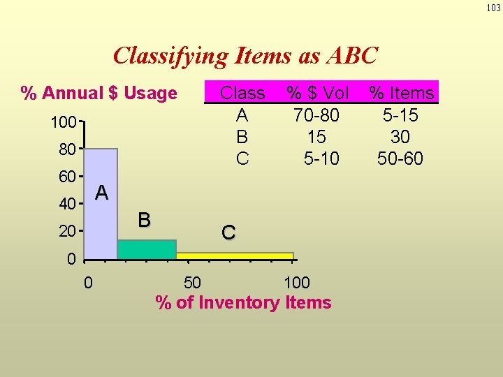
103 Classifying Items as ABC Class A B C % Annual $ Usage 100 80 60 % $ Vol 70 -80 15 5 -10 A 40 B 20 C 0 0 50 100 % of Inventory Items % Items 5 -15 30 50 -60

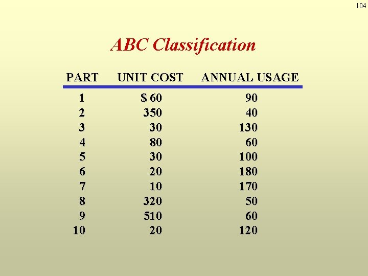
104 ABC Classification PART UNIT COST ANNUAL USAGE 1 2 3 4 5 6 7 8 9 10 $ 60 350 30 80 30 20 10 320 510 20 90 40 130 60 100 180 170 50 60 120

105 ABC Classification PART 9 8 2 1 4 3 6 5 10 7 TOTAL % OF TOTAL PART UNIT ANNUAL USAGE VALUECOSTQUANTITY % CUMMULATIVE $30, 600 1 16, 000 2 14, 000 3 5, 400 4 4, 800 5 3, 900 3, 600 6 3, 000 7 2, 400 8 1, 700 9 $85, 400 10 35. 9 $ 60 18. 7 350 16. 4 30 6. 3 5. 680 4. 630 4. 220 3. 510 2. 8 320 2. 0 510 20 6. 0 5. 0 4. 0 9. 0 6. 0 10. 0 18. 0 13. 0 12. 0 17. 0 90 40 130 60 100 180 170 50 60 120 6. 0 11. 0 15. 0 24. 0 30. 0 40. 0 58. 0 71. 0 83. 0 100. 0

106 ABC Classification PART 9 8 2 1 4 3 6 5 10 7 TOTAL % OF TOTAL PART UNIT ANNUAL USAGE VALUECOSTQUANTITY % CUMMULATIVE $30, 600 1 16, 000 2 14, 000 3 5, 400 4 4, 800 5 3, 900 3, 600 6 3, 000 7 2, 400 8 1, 700 9 $85, 400 10 35. 9 $ 60 18. 7 350 16. 4 30 6. 3 5. 680 4. 630 4. 220 3. 510 2. 8 320 2. 0 510 20 6. 0 5. 0 4. 0 9. 0 6. 0 10. 0 18. 0 13. 0 12. 0 17. 0 90 A 40 130 60 B 100 180 170 C 50 60 120 6. 0 11. 0 15. 0 24. 0 30. 0 40. 0 58. 0 71. 0 83. 0 100. 0

107 ABC Classification PART TOTAL % OF TOTAL PART UNIT ANNUAL USAGE VALUECOSTQUANTITY % CUMMULATIVE 9 $30, 600 1 8 16, 000 2 2 14, 000 3 1 CLASS 5, 400 4 4 4, 800 A 3, 900 5 3 B 3, 600 6 6 C 3, 000 5 7 10 2, 400 8 7 1, 700 9 $85, 400 10 35. 9 6. 0 $ 60 18. 7 5. 0 350 16. 4 % OF TOTAL 4. 0 30 6. 3 ITEMS VALUE 9. 0 5. 680 6. 0 9, 8, 2 4. 630 71. 010. 0 1, 4, 3 4. 220 16. 518. 0 6, 5, 10, 3. 5 7 12. 513. 0 10 2. 8 12. 0 320 2. 0 17. 0 510 20 6. 0 90 11. 0 A 40 15. 0 % OF TOTAL 130 24. 0 QUANTITY 60 B 15. 030. 0 100 40. 0 180 25. 058. 0 60. 071. 0 170 C 83. 0 50 100. 0 60 120

108 ABC Classification C 100 – B % of Value 80 – 60 – A 40 – 20 – 0 | 20 | | 40 60 % of Quantity | 80 | 100

109 Inventory Accuracy and Cycle Counting • Inventory accuracy refers to how well the inventory records agree with physical count. • Physically counting a sample of total inventory on a regular basis • Used often with ABC classification – A items counted most often (e. g. , daily)

110 Advantages of Cycle Counting • Eliminates shutdown and interruption of production necessary for annual physical inventories • Eliminates annual inventory adjustments • Provides trained personnel to audit the accuracy of inventory • Allows the cause of errors to be identified and remedial action to be taken • Maintains accurate inventory records

111 Last Words Inventories have certain functions. But too much inventory - Tends to hide problems - Costly to maintain So it is desired • Reduce lot sizes • Reduce safety stocks