1 Instant Analyses in AFNI and SUMA SUMA

– 1– Instant Analyses in AFNI and SUMA: SUMA Clusters and Correlations Data for this presentation: AFNI_data 5/ directory All data herein from Alex Martin, et al. [NIMH IRP]

– 2– AFNI “Insta” Functions • 3 new capabilities added to the interactive AFNI • Each one: compute new dataset volumes instantly to replace the Overlay volume for image viewing • Clusters = interactive clustering § remove clusters below a user-chosen size § display a table of clusters • Insta. Corr = interactive exploration of inter-voxel time series correlation § choose a seed voxel and see correlation map § SUMA version also exists • Insta. Calc = interactive version of 3 dcalc § e. g. , display ratio of 2 datasets

– 3– Clusters: Setup • Open Define Overlay, choose Clusters from menu in top right corner • Then press Clusterize to get the clusters control menu

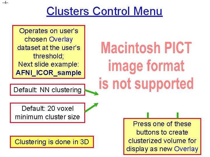
– 4– Clusters Control Menu Operates on user’s chosen Overlay dataset at the user’s threshold; Next slide example: AFNI_ICOR_sample Default: NN clustering Default: 20 voxel minimum cluster size Clustering is done in 3 D Press one of these buttons to create clusterized volume for display as new Overlay

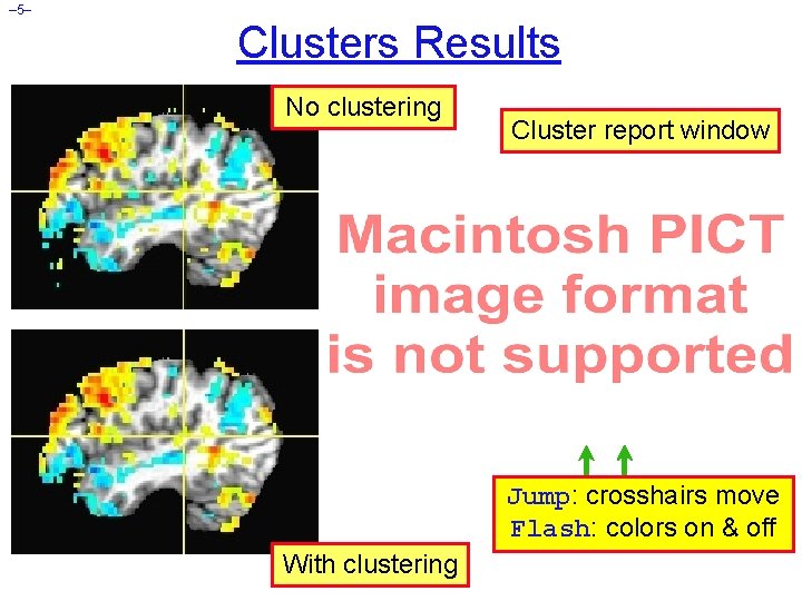
– 5– Clusters Results No clustering Cluster report window Jump: crosshairs move Flash: colors on & off With clustering

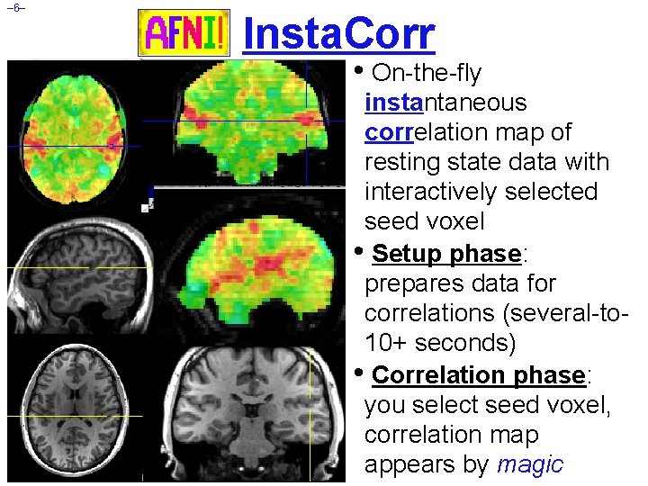
– 6– Insta. Corr • On-the-fly instantaneous correlation map of resting state data with interactively selected seed voxel • Setup phase: prepares data for correlations (several-to 10+ seconds) • Correlation phase: you select seed voxel, correlation map appears by magic

– 7– Insta. Corr: Outline of 2 Phases • Setup phase: Masking: user-selected or Automask § Bandpass and other filtering of voxel time series § Blurring inside mask = the slowest part • Correlation phase: § Correlate selected seed voxel time series with all other prepared voxel time series § Make new dataset, if needed, to store results § Save seed time series for graphing § Redisplay color overlay § Optional: compute FDR curve for correlations § o Calculation is slow, so FDR is not turned on by default

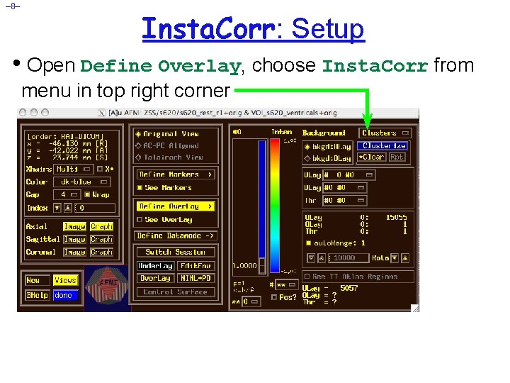
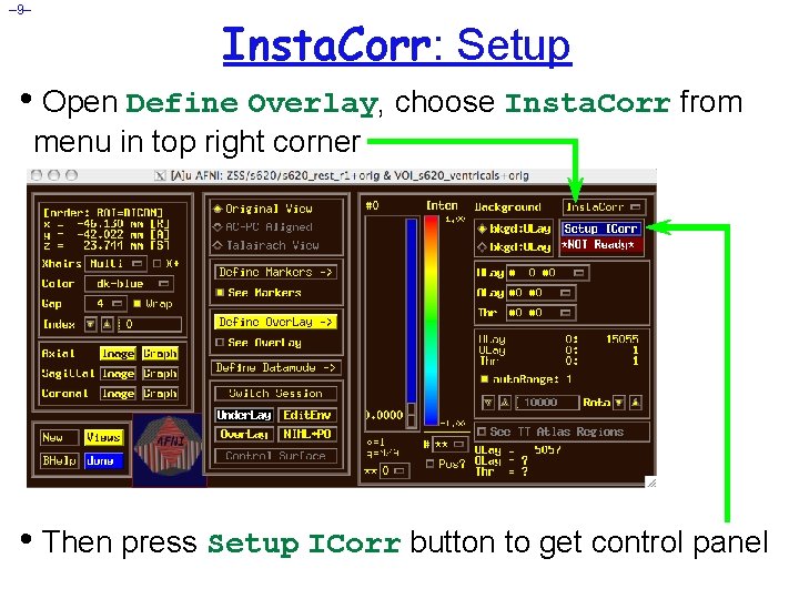
– 8– Insta. Corr: Setup • Open Define Overlay, choose Insta. Corr from menu in top right corner

– 9– Insta. Corr: Setup • Open Define Overlay, choose Insta. Corr from menu in top right corner • Then press Setup ICorr button to get control panel

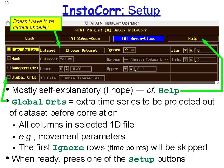
– 10– Insta. Corr: Setup Doesn’t have to be current underlay • Mostly self-explanatory (I hope) — cf. Help • Global Orts = extra time series to be projected out of dataset before correlation § All columns in selected 1 D file § e. g. , movement parameters § The first Ignore rows (time points) will be skipped • When ready, press one of the Setup buttons

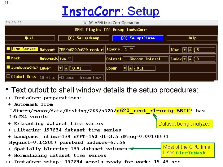
– 11– Insta. Corr: Setup • Text output to shell window details the setup procedures: ++ Insta. Corr preparations: + Automask from '/Users/rwcox/data/Resting/ZSS/s 620_rest_r 1+orig. BRIK' has 197234 voxels + Extracting dataset time series Dataset being analyzed + Filtering 197234 dataset time series + bandpass: ntime=139 n. FFT=160 dt=3. 5 d. Freq=0. 00178571 Nyquist=0. 142857 passband indexes=6. . 56 Most of the CPU time: + Spatially blurring 139 dataset volumes Uses Blur. In. Mask + Normalizing dataset time series ++ Insta. Corr setup: 197234 voxels ready for work: 15. 43 sec

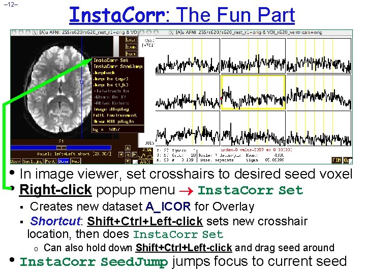
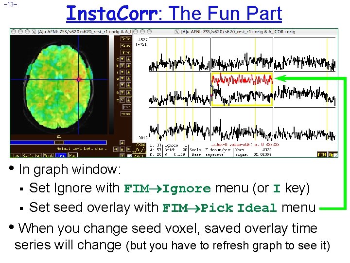
Insta. Corr: The Fun Part – 12– • In image viewer, set crosshairs to desired seed voxel • Right-click popup menu Insta. Corr Set Creates new dataset A_ICOR for Overlay § Shortcut: Shift+Ctrl+Left-click sets new crosshair location, then does Insta. Corr Set § o Can also hold down Shift+Ctrl+Left-click and drag seed around • Insta. Corr Seed. Jump jumps focus to current seed

Insta. Corr: The Fun Part – 13– • In graph window: § § Set Ignore with FIM Ignore menu (or I key) Set seed overlay with FIM Pick Ideal menu • When you change seed voxel, saved overlay time series will change (but you have to refresh graph to see it)

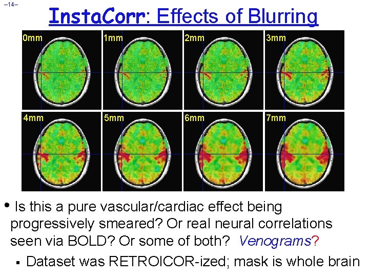
Insta. Corr: Effects of Blurring – 14– 0 mm 1 mm 2 mm 3 mm 4 mm 5 mm 6 mm 7 mm • Is this a pure vascular/cardiac effect being progressively smeared? Or real neural correlations seen via BOLD? Or some of both? Venograms? § Dataset was RETROICOR-ized; mask is whole brain

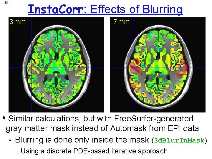
Insta. Corr: Effects of Blurring – 15– 3 mm 7 mm • Similar calculations, but with Free. Surfer-generated gray matter mask instead of Automask from EPI data § Blurring is done only inside the mask (3 d. Blur. In. Mask) o Using a discrete PDE-based iterative approach

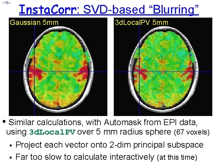
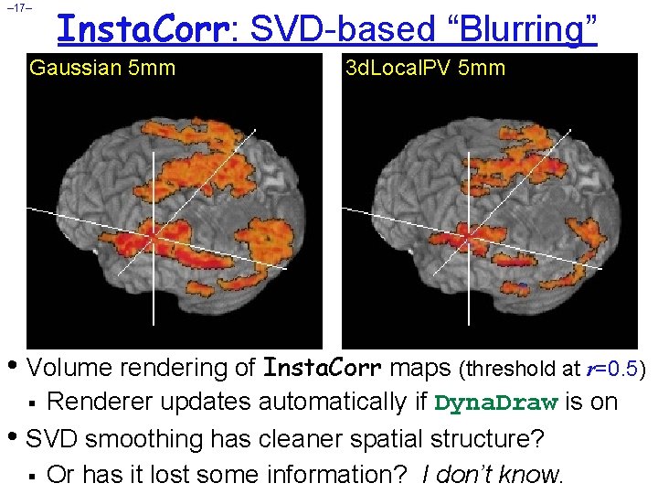
– 16– Insta. Corr: SVD-based “Blurring” Gaussian 5 mm 3 d. Local. PV 5 mm • Similar calculations, with Automask from EPI data, using 3 d. Local. PV over 5 mm radius sphere (67 voxels) § § Project each vector onto 2 -dim principal subspace Far too slow to calculate interactively (at this time)

– 17– Insta. Corr: SVD-based “Blurring” Gaussian 5 mm 3 d. Local. PV 5 mm • Volume rendering of Insta. Corr maps (threshold at r=0. 5) Renderer updates automatically if Dyna. Draw is on • SVD smoothing has cleaner spatial structure? § Or has it lost some information? I don’t know. §

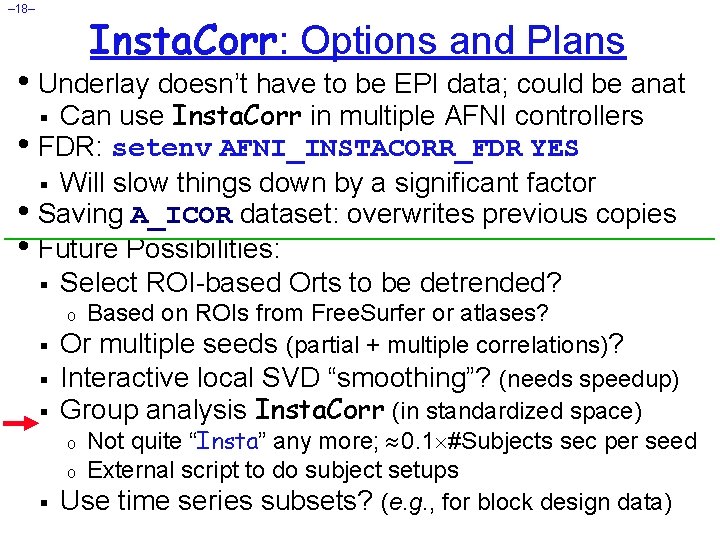
– 18– Insta. Corr: Options and Plans • Underlay doesn’t have to be EPI data; could be anat Can use Insta. Corr in multiple AFNI controllers • FDR: setenv AFNI_INSTACORR_FDR YES § Will slow things down by a significant factor • Saving A_ICOR dataset: overwrites previous copies • Future Possibilities: § Select ROI-based Orts to be detrended? § Based on ROIs from Free. Surfer or atlases? Or multiple seeds (partial + multiple correlations)? Interactive local SVD “smoothing”? (needs speedup) Group analysis Insta. Corr (in standardized space) o Not quite “Insta” any more; 0. 1 #Subjects sec per seed o External script to do subject setups Use time series subsets? (e. g. , for block design data) o § §

– 19– Group Insta. Corr • If you have a robust enough system (multiple CPUs, several gigabytes of RAM), you can explore the group analysis of resting state seed-based correlations • Setup Phase: § Unlike individual Insta. Corr, the setup is done outside the AFNI GUI with command line programs § Step 1: transform all time series datasets to standard space = @auto_tlrc and adwarp § Step 2: filter and blur all time series dataset = 3 d. Bandpass § Step 3: collect groups of time series datasets into one big file = 3 d. Setup. Group. In. Corr • Interactive Phase: point-and-click to set seed voxel 31 Dec 2009

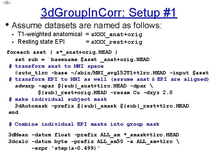
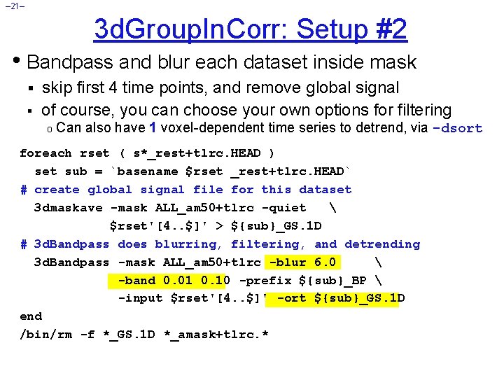
– 20– 3 d. Group. In. Corr: Setup #1 • Assume datasets are named as follows: § § T 1 -weighted anatomical = s. XXX_anat+orig Resting state EPI = s. XXX_rest+orig foreach aset ( s*_anat+orig. HEAD ) set sub = `basename $aset _anat+orig. HEAD` # transform anat to MNI space @auto_tlrc -base ~/abin/MNI_avg 152 T 1+tlrc. HEAD -input $aset # transform EPI to MNI as well (assume anat & EPI are aligned) adwarp -apar ${sub}_anat+tlrc. HEAD -dpar ${sub}_rest+orig. HEAD -resam Cu -dxyz 2. 0 # make individual subject mask 3 d. Automask -prefix ${sub}_amask ${sub}_rest+tlrc. HEAD end # Combine individual EPI masks into group mask 3 d. Mean -datum float -prefix ALL_am *_amask+tlrc. HEAD 3 dcalc -datum byte -prefix ALL_am 50 -a ALL_am+tlrc -expr 'step(a-0. 499)'

– 21– 3 d. Group. In. Corr: Setup #2 • Bandpass and blur each dataset inside mask § skip first 4 time points, and remove global signal § of course, you can choose your own options for filtering o Can also have 1 voxel-dependent time series to detrend, via -dsort foreach rset ( s*_rest+tlrc. HEAD ) set sub = `basename $rset _rest+tlrc. HEAD` # create global signal file for this dataset 3 dmaskave -mask ALL_am 50+tlrc -quiet $rset'[4. . $]' > ${sub}_GS. 1 D # 3 d. Bandpass does blurring, filtering, and detrending 3 d. Bandpass -mask ALL_am 50+tlrc -blur 6. 0 -band 0. 01 0. 10 -prefix ${sub}_BP -input $rset'[4. . $]' -ort ${sub}_GS. 1 D end /bin/rm -f *_GS. 1 D *_amask+tlrc. *

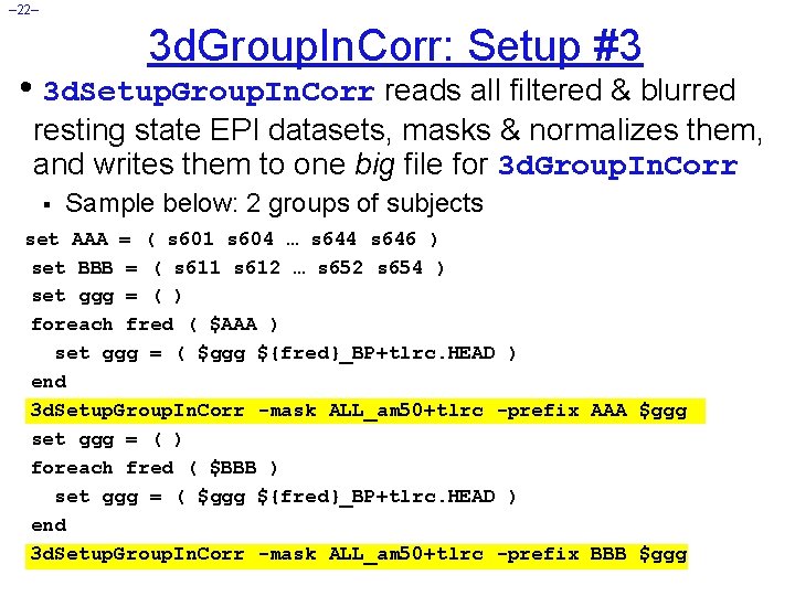
– 22– 3 d. Group. In. Corr: Setup #3 • 3 d. Setup. Group. In. Corr reads all filtered & blurred resting state EPI datasets, masks & normalizes them, and writes them to one big file for 3 d. Group. In. Corr § Sample below: 2 groups of subjects set AAA = ( s 601 s 604 … s 644 s 646 ) set BBB = ( s 611 s 612 … s 652 s 654 ) set ggg = ( ) foreach fred ( $AAA ) set ggg = ( $ggg ${fred}_BP+tlrc. HEAD ) end 3 d. Setup. Group. In. Corr -mask ALL_am 50+tlrc -prefix AAA $ggg set ggg = ( ) foreach fred ( $BBB ) set ggg = ( $ggg ${fred}_BP+tlrc. HEAD ) end 3 d. Setup. Group. In. Corr -mask ALL_am 50+tlrc -prefix BBB $ggg

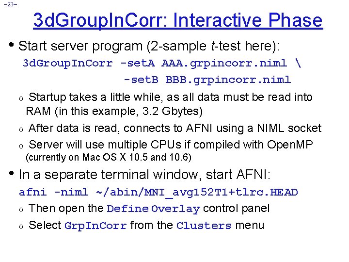
– 23– 3 d. Group. In. Corr: Interactive Phase • Start server program (2 -sample t-test here): 3 d. Group. In. Corr -set. A AAA. grpincorr. niml -set. B BBB. grpincorr. niml Startup takes a little while, as all data must be read into RAM (in this example, 3. 2 Gbytes) o After data is read, connects to AFNI using a NIML socket o Server will use multiple CPUs if compiled with Open. MP o (currently on Mac OS X 10. 5 and 10. 6) • In a separate terminal window, start AFNI: afni -niml ~/abin/MNI_avg 152 T 1+tlrc. HEAD o Then open the Define Overlay control panel o Select Grp. In. Corr from the Clusters menu

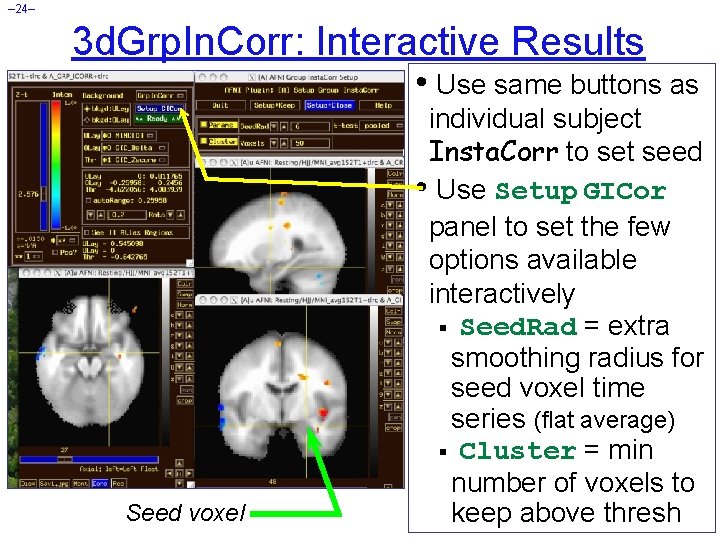
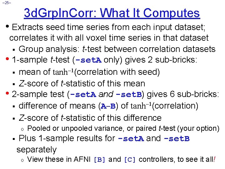
– 24– 3 d. Grp. In. Corr: Interactive Results • Use same buttons as Seed voxel individual subject Insta. Corr to set seed • Use Setup GICor panel to set the few options available interactively § Seed. Rad = extra smoothing radius for seed voxel time series (flat average) § Cluster = min number of voxels to keep above thresh

– 25– 3 d. Grp. In. Corr: What It Computes • Extracts seed time series from each input dataset; correlates it with all voxel time series in that dataset § Group analysis: t-test between correlation datasets • 1 -sample t-test (-set. A only) gives 2 sub-bricks: § mean of tanh 1(correlation with seed) § Z-score of t-statistic of this mean • 2 -sample test (-set. A and -set. B) gives 6 sub-bricks: § difference of means (A B) of tanh 1(correlation) § Z-score of t-statistic of this difference o § Pooled or unpooled variance, or paired t-test (your option) Plus 1 -sample results for -set. A and -set. B separately o View these in AFNI [B] and [C] controllers, to see it all!

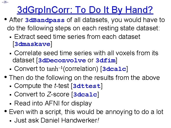
– 26– 3 d. Grp. In. Corr: To Do It By Hand? • After 3 d. Bandpass of all datasets, you would have to do the following steps on each resting state dataset: § Extract seed time series from each dataset [3 dmaskave] § Correlate seed time series with all voxels from its dataset [3 d. Deconvolve or 3 dfim] § Convert to tanh 1(correlation) [3 dcalc] • Then do the following on the results from the above § Compute the t-test [3 dttest] § Convert to Z-score [3 dcalc] § Read into AFNI for display • Even with a script, this would be annoying to do a lot § Just ask Daniel Handwerker!

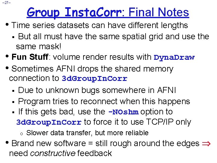
– 27– Group Insta. Corr: Final Notes • Time series datasets can have different lengths But all must have the same spatial grid and use the same mask! • Fun Stuff: volume render results with Dyna. Draw • Sometimes AFNI drops the shared memory connection to 3 d. Group. In. Corr § Due to unknown bugs somewhere in AFNI § Program tries to reconnect when this happens § If this gets bad, use the -NOshm option to 3 d. Group. In. Corr to force it to use TCP/IP only § o Slower data transfer, but more reliable • Brand new software = still rough around the edges need constructive feedback

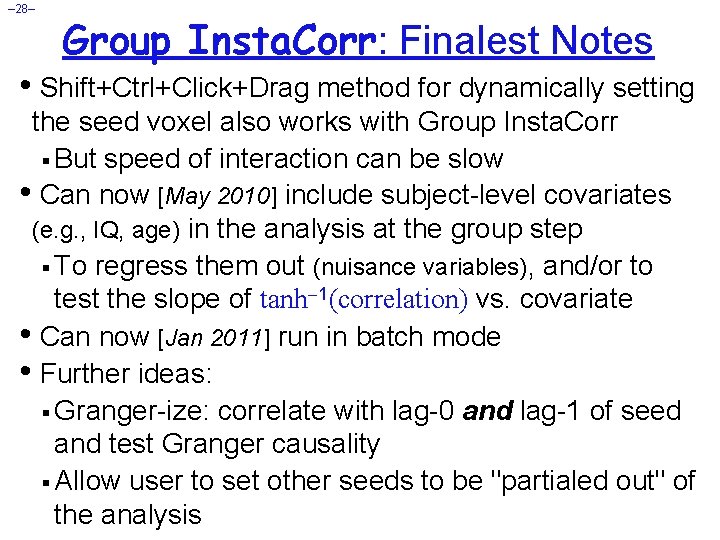
– 28– Group Insta. Corr: Finalest Notes • Shift+Ctrl+Click+Drag method for dynamically setting the seed voxel also works with Group Insta. Corr § But speed of interaction can be slow • Can now [May 2010] include subject-level covariates (e. g. , IQ, age) in the analysis at the group step § To regress them out (nuisance variables), and/or to test the slope of tanh 1(correlation) vs. covariate • Can now [Jan 2011] run in batch mode • Further ideas: § Granger-ize: correlate with lag-0 and lag-1 of seed and test Granger causality § Allow user to set other seeds to be "partialed out" of the analysis

– 29– Insta. Calc: Dataset Calculator • Open Define Overlay, choose Insta. Calc from menu in top right corner • Then press Setup ICalc button to get control panel

– 30– Insta. Calc: Setup • Select datasets with Choose Dataset buttons and sub-bricks with the [-] controls • Enter symbolic expression • Press Compute Insta. Calc • Creates new 1 -brick dataset A_ICALC for Overlay § voxel-by-voxel calculations §

– 31– Insta. Corr • Similar in concept to AFNI Insta. Corr but requires external pre-processing of time series datasets § Removal of baseline, projection to surface, blurring • In the AFNI_data 5/ directory, run the script tcsh. /@run_REST_demo § starts SUMA with 2 hemispheres § loads pre-processed datasets into SUMA § sets up SUMA’s Insta. Corr • After all the setup is ready, right-clicking on the surface will do the Insta. Corr calculations • 3 d. Group. In. Corr also works with SUMA

– 32– Insta. Corr: Sample • Seed voxel and Seed voxel time series graph