1 Historical Simulation ValueatRisk and Expected Shortfall Elements

1 Historical Simulation, Value-at-Risk, and Expected Shortfall Elements of Financial Risk Management Chapter 2 Peter Christoffersen Elements of Financial Risk Management Second Edition © 2012 by Peter Christoffersen

Overview Objectives • Introduce the most commonly used method for computing Va. R, namely Historical Simulation and discuss the pros and cons of this method. • Discuss the pros and cons of the V a. R risk measure • Consider the Expected Shortfall, ES, alternative. Elements of Financial Risk Management Second Edition © 2012 by Peter Christoffersen 2

Chapter is organized as follows: • Introduction of the historical simulation (HS) method and its pros and cons. • Introduction of the weighted historical simulation (WHS). We then compare HS and WHS during the 1987 crash. • Comparison of the performance of HS and Risk. Metrics during the 2008 -2009 financial crisis. • Then we simulate artificial return data and assess the HS Va. R on this data. • Compare the Va. R risk measure with ES. Elements of Financial Risk Management Second Edition © 2012 by Peter Christoffersen 3

Defining Historical Simulation • Let today be day t. Consider a portfolio of n assets. If we today own Ni, t units or shares of asset i then the value of the portfolio today is • We use today’s portfolio holdings but historical asset prices to compute yesterday’s pseudo portfolio value as Elements of Financial Risk Management Second Edition © 2012 by Peter Christoffersen 4

Defining Historical Simulation • This is a pseudo value because the units of each asset held typically changes over time. The pseudo log return can now be defined as • Consider the availability of a past sequence of m daily hypothetical portfolio returns, calculated using past prices of the underlying assets of the portfolio, but using today’s portfolio weights, call it {RPF, t+1 -t}mt=1 Elements of Financial Risk Management Second Edition © 2012 by Peter Christoffersen 5

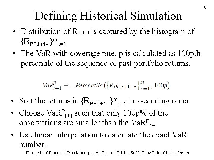
Defining Historical Simulation • Distribution of RPF, t+1 is captured by the histogram of {RPF, t+1 -t}mt=1 • The Va. R with coverage rate, p is calculated as 100 pth percentile of the sequence of past portfolio returns. • Sort the returns in {RPF, t+1 -t}mt=1 in ascending order • Choose Va. RPt+1 such that only 100 p% of the observations are smaller than the Va. RPt+1 • Use linear interpolation to calculate the exact Va. R number. Elements of Financial Risk Management Second Edition © 2012 by Peter Christoffersen 6

Pros and Cons of HS Pros • the ease with which it is implemented. • its model-free nature. Cons • It is very easy to implement. No numerical optimization has to be performed. • It is model-free. It does not rely on any particular parametric model such as a Risk. Metrics model. Elements of Financial Risk Management Second Edition © 2012 by Peter Christoffersen 7

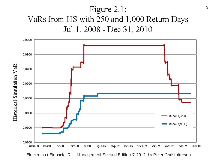
Issues with model free nature of HS How large should m be? • If m is too large, then the most recent observations will carry very little weight, and the Va. R will tend to look very smooth over time. • If m is too small, then the sample may not include enough large losses to enable the risk manager to calculate Va. R with any precision. • To calculate 1% Va. Rs with any degree of precision for the next 10 days, HS technique needs a large m value Elements of Financial Risk Management Second Edition © 2012 by Peter Christoffersen 8

Figure 2. 1: Va. Rs from HS with 250 and 1, 000 Return Days Jul 1, 2008 - Dec 31, 2010 9 0, 0900 Historical Simulation Va. R 0, 0800 0, 0700 0, 0600 0, 0500 0, 0400 HS-Va. R(250) HS-Va. R(1000) 0, 0300 0, 0200 июн-08 июл-08 сен-08 окт-08 дек-08 фев-09 мар-09 май-09 июл-09 авг-09 окт-09 дек-09 Elements of Financial Risk Management Second Edition © 2012 by Peter Christoffersen янв-10

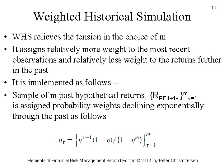
Weighted Historical Simulation 10 • WHS relieves the tension in the choice of m • It assigns relatively more weight to the most recent observations and relatively less weight to the returns further in the past • It is implemented as follows – • Sample of m past hypothetical returns, {RPF, t+1 -t}mt=1 is assigned probability weights declining exponentially through the past as follows Elements of Financial Risk Management Second Edition © 2012 by Peter Christoffersen

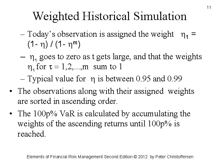
Weighted Historical Simulation – Today’s observation is assigned the weight 1 = (1 - ) / (1 - m) – t goes to zero as t gets large, and that the weights t for t = 1, 2, . . . , m sum to 1 – Typical value for is between 0. 95 and 0. 99 • The observations along with their assigned weights are sorted in ascending order. • The 100 p% Va. R is calculated by accumulating the weights of the ascending returns until 100 p% is reached. Elements of Financial Risk Management Second Edition © 2012 by Peter Christoffersen 11

Pros and Cons of WHS Pros • Once is chosen, WHS does not require estimation and becomes easy to implement • It’s weighting function builds dynamics into the WHS technique • The weighting function also makes the choice of m somewhat less crucial. • WHS responds quickly to large losses Elements of Financial Risk Management Second Edition © 2012 by Peter Christoffersen 12

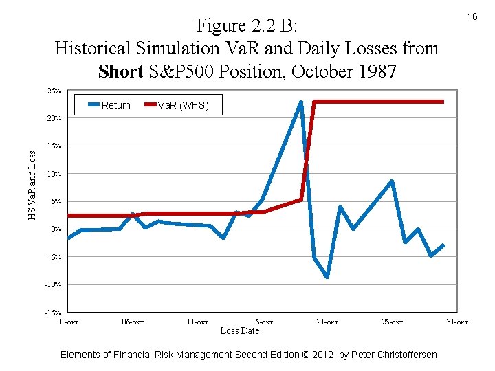
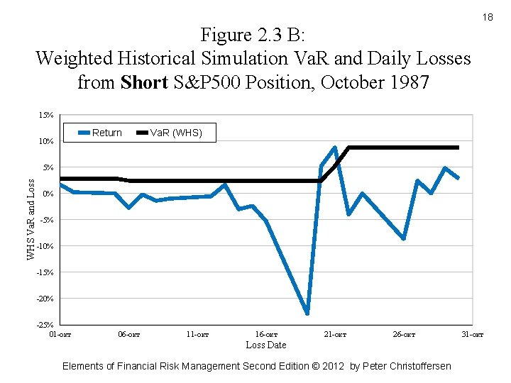
Pros and Cons of WHS Cons • No guidance is given on how to choose η • Effect on the weighting scheme of positive versus negative past returns • If we are short the market, a market crash has no impact on our Va. R. WHS does not respond to large gains • the multiday Va. R requires a large amount of past daily return data, which is not easy to obtain. Elements of Financial Risk Management Second Edition © 2012 by Peter Christoffersen 13

Advantages of Risk Metrics model • It can pick up the increase in market variance from the crash regardless of whether the crash meant a gain or a loss • In this model, returns are squared and losses and gains are treated as having the same impact on tomorrow’s variance and therefore on the portfolio risk. Elements of Financial Risk Management Second Edition © 2012 by Peter Christoffersen 14

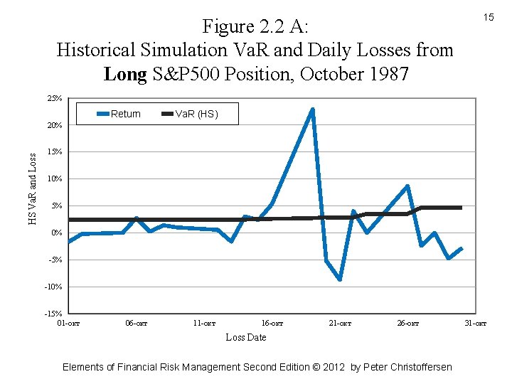
Figure 2. 2 A: Historical Simulation Va. R and Daily Losses from Long S&P 500 Position, October 1987 15 25% Return Va. R (HS) HS Va. R and Loss 20% 15% 10% 5% 0% -5% -10% -15% 01 -окт 06 -окт 11 -окт 16 -окт 21 -окт 26 -окт Loss Date Elements of Financial Risk Management Second Edition © 2012 by Peter Christoffersen 31 -окт

Figure 2. 2 B: Historical Simulation Va. R and Daily Losses from Short S&P 500 Position, October 1987 16 25% Return Va. R (WHS) 20% HS Va. R and Loss 15% 10% 5% 0% -5% -10% -15% 01 -окт 06 -окт 11 -окт 16 -окт Loss Date 21 -окт 26 -окт Elements of Financial Risk Management Second Edition © 2012 by Peter Christoffersen 31 -окт

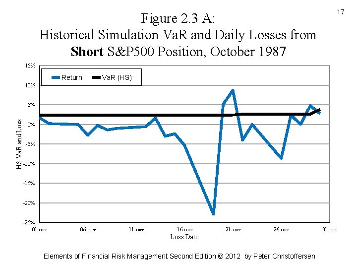
Figure 2. 3 A: Historical Simulation Va. R and Daily Losses from Short S&P 500 Position, October 1987 17 15% Return Va. R (HS) 10% HS Va. R and Loss 5% 0% -5% -10% -15% -20% -25% 01 -окт 06 -окт 11 -окт 16 -окт 21 -окт 26 -окт Loss Date Elements of Financial Risk Management Second Edition © 2012 by Peter Christoffersen 31 -окт

18 Figure 2. 3 B: Weighted Historical Simulation Va. R and Daily Losses from Short S&P 500 Position, October 1987 15% Return 10% Va. R (WHS) WHS Va. R and Loss 5% 0% -5% -10% -15% -20% -25% 01 -окт 06 -окт 11 -окт 16 -окт 21 -окт 26 -окт Loss Date Elements of Financial Risk Management Second Edition © 2012 by Peter Christoffersen 31 -окт

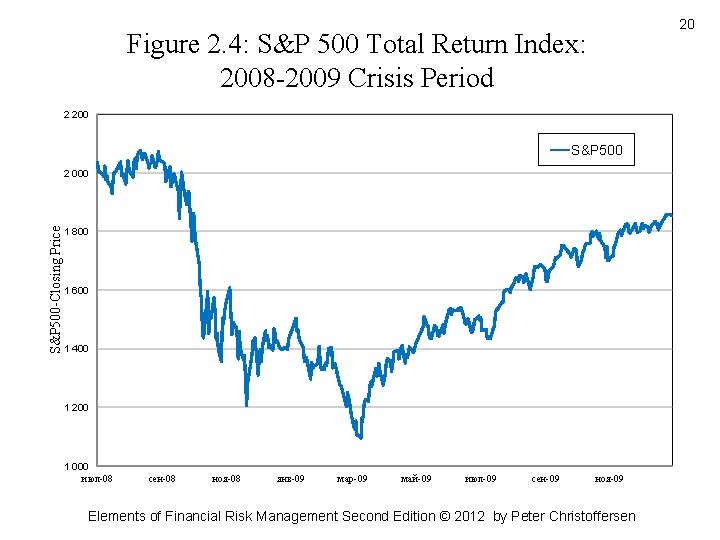
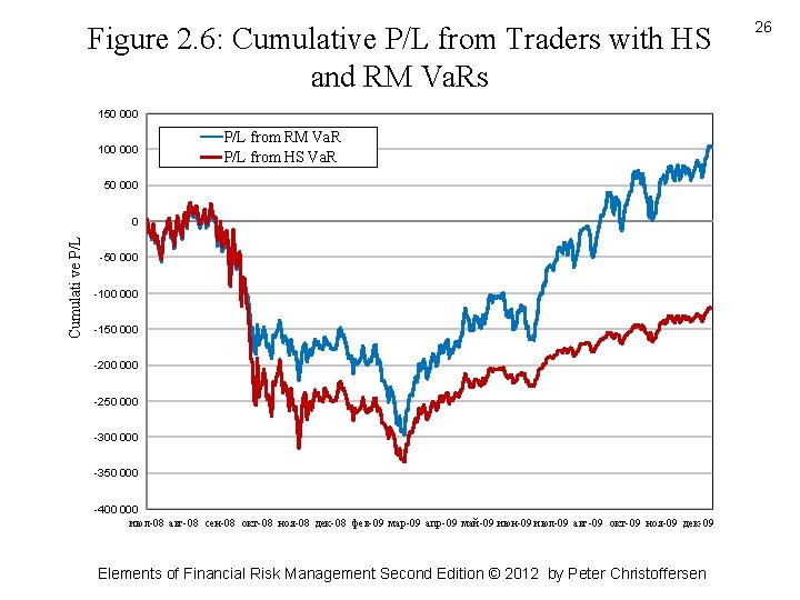
Evidence from the 2008 -2009 Crisis • We consider the daily closing prices for a total return index of the S&P 500 starting in July 2008 and ending in December 2009. • The index lost almost half its value between July 2008 and the market bottom in March 2009. • The recovery in the index starting in March 2009 continued through the end of 2009. Elements of Financial Risk Management Second Edition © 2012 by Peter Christoffersen 19

20 Figure 2. 4: S&P 500 Total Return Index: 2008 -2009 Crisis Period 2 200 S&P 500 -Closing Price 2 000 1 800 1 600 1 400 1 200 1 000 июл-08 сен-08 ноя-08 янв-09 мар-09 май-09 июл-09 сен-09 ноя-09 Elements of Financial Risk Management Second Edition © 2012 by Peter Christoffersen

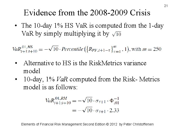
Evidence from the 2008 -2009 Crisis • The 10 -day 1% HS Va. R is computed from the 1 -day Va. R by simply multiplying it by • Alternative to HS is the Risk. Metrics variance model • 10 -day, 1% Va. R computed from the Risk- Metrics model is as follows: Elements of Financial Risk Management Second Edition © 2012 by Peter Christoffersen 21

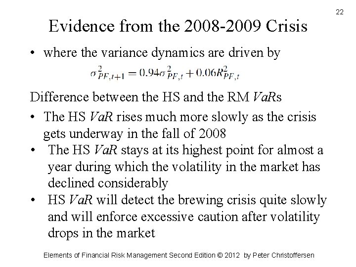
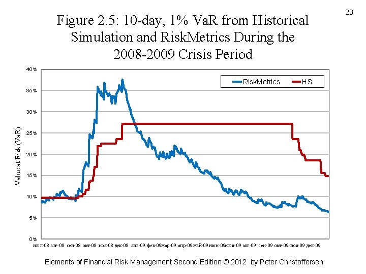
Evidence from the 2008 -2009 Crisis • where the variance dynamics are driven by Difference between the HS and the RM Va. Rs • The HS Va. R rises much more slowly as the crisis gets underway in the fall of 2008 • The HS Va. R stays at its highest point for almost a year during which the volatility in the market has declined considerably • HS Va. R will detect the brewing crisis quite slowly and will enforce excessive caution after volatility drops in the market Elements of Financial Risk Management Second Edition © 2012 by Peter Christoffersen 22

Figure 2. 5: 10 -day, 1% Va. R from Historical Simulation and Risk. Metrics During the 2008 -2009 Crisis Period 40% Risk. Metrics HS 35% Value at Risk (Va. R) 30% 25% 20% 15% 10% 5% 0% июл-08 авг-08 сен-08 окт-08 ноя-08 дек-08 янв-09 фев-09 мар-09 апр-09 май-09 июн-09 июл-09 авг-09 сен-09 окт-09 ноя-09 дек-09 Elements of Financial Risk Management Second Edition © 2012 by Peter Christoffersen 23

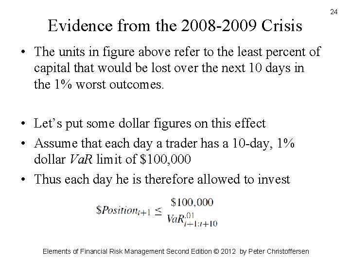
Evidence from the 2008 -2009 Crisis • The units in figure above refer to the least percent of capital that would be lost over the next 10 days in the 1% worst outcomes. • Let’s put some dollar figures on this effect • Assume that each day a trader has a 10 -day, 1% dollar Va. R limit of $100, 000 • Thus each day he is therefore allowed to invest Elements of Financial Risk Management Second Edition © 2012 by Peter Christoffersen 24

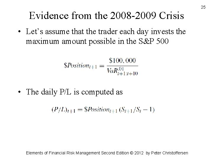
Evidence from the 2008 -2009 Crisis • Let’s assume that the trader each day invests the maximum amount possible in the S&P 500 • The daily P/L is computed as Elements of Financial Risk Management Second Edition © 2012 by Peter Christoffersen 25

Figure 2. 6: Cumulative P/L from Traders with HS and RM Va. Rs 150 000 100 000 P/L from RM Va. R P/L from HS Va. R 50 000 Cumulati ve P/L 0 -50 000 -100 000 -150 000 -200 000 -250 000 -300 000 -350 000 -400 000 июл-08 авг-08 сен-08 окт-08 ноя-08 дек-08 фев-09 мар-09 апр-09 май-09 июн-09 июл-09 авг-09 окт-09 ноя-09 дек-09 Elements of Financial Risk Management Second Edition © 2012 by Peter Christoffersen 26

Evidence from the 2008 -2009 Crisis 27 Performance difference between HS and RM Va. Rs • The RM trader will lose less in the fall of 2008 and earn much more in 2009. • The HS trader takes more losses in the fall of 2008 and is not allowed to invest sufficiently in the market in 2009 • The HS Va. R reacts too slowly to increases in volatility as well as to decreases in volatility. Elements of Financial Risk Management Second Edition © 2012 by Peter Christoffersen

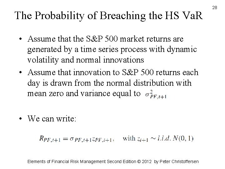
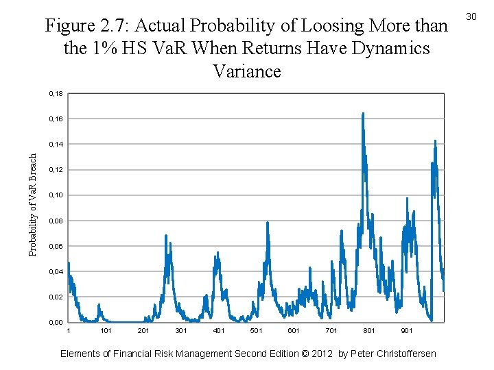
The Probability of Breaching the HS Va. R • Assume that the S&P 500 market returns are generated by a time series process with dynamic volatility and normal innovations • Assume that innovation to S&P 500 returns each day is drawn from the normal distribution with mean zero and variance equal to • We can write: Elements of Financial Risk Management Second Edition © 2012 by Peter Christoffersen 28

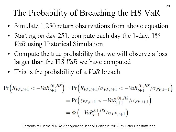
The Probability of Breaching the HS Va. R 29 • Simulate 1, 250 return observations from above equation • Starting on day 251, compute each day the 1 -day, 1% Va. R using Historical Simulation • Compute the true probability that we will observe a loss larger than the HS Va. R we have computed • This is the probability of a Va. R breach Elements of Financial Risk Management Second Edition © 2012 by Peter Christoffersen

Figure 2. 7: Actual Probability of Loosing More than the 1% HS Va. R When Returns Have Dynamics Variance 0, 18 0, 16 Probability of Va. R Breach 0, 14 0, 12 0, 10 0, 08 0, 06 0, 04 0, 02 0, 00 1 101 201 301 401 501 601 701 801 901 Elements of Financial Risk Management Second Edition © 2012 by Peter Christoffersen 30

The Probability of Breaching the HS Va. R • where is the cumulative density function for a standard normal random variable. • If the HS Va. R model had been accurate then this plot should show a roughly flat line at 1% • Here we see numbers as high as 16% and numbers very close to 0% • The HS Va. R will overestimate risk when true market volatility is low, which will generate a low probability of a Va. R breach • HS will underestimate risk when true volatility is high in which case the Va. R breach volatility will be high Elements of Financial Risk Management Second Edition © 2012 by Peter Christoffersen 31

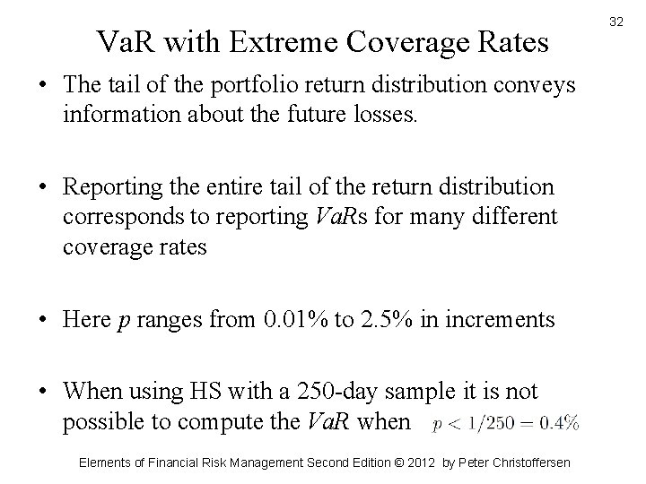
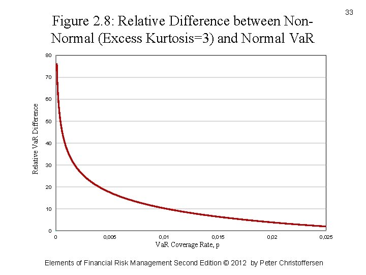
Va. R with Extreme Coverage Rates • The tail of the portfolio return distribution conveys information about the future losses. • Reporting the entire tail of the return distribution corresponds to reporting Va. Rs for many different coverage rates • Here p ranges from 0. 01% to 2. 5% in increments • When using HS with a 250 -day sample it is not possible to compute the Va. R when Elements of Financial Risk Management Second Edition © 2012 by Peter Christoffersen 32

33 Figure 2. 8: Relative Difference between Non. Normal (Excess Kurtosis=3) and Normal Va. R 80 70 Relative Va. R Difference 60 50 40 30 20 10 0 0 0, 005 0, 015 0, 025 Va. R Coverage Rate, p Elements of Financial Risk Management Second Edition © 2012 by Peter Christoffersen

Va. R with Extreme Coverage Rates • Note that (from the above figure) as p gets close to zero the nonnormal Va. R gets much larger than the normal Va. R • When p = 0. 025 there is almost no difference between the two Va. Rs even though the underlying distributions are different Elements of Financial Risk Management Second Edition © 2012 by Peter Christoffersen 34

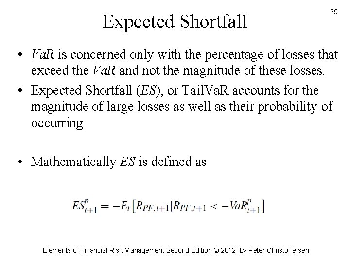
Expected Shortfall 35 • Va. R is concerned only with the percentage of losses that exceed the Va. R and not the magnitude of these losses. • Expected Shortfall (ES), or Tail. Va. R accounts for the magnitude of large losses as well as their probability of occurring • Mathematically ES is defined as Elements of Financial Risk Management Second Edition © 2012 by Peter Christoffersen

Expected Shortfall 36 • The negative signs in front of the expectation and the Va. R are needed because the ES and the Va. R are defined as positive numbers • The ES tells us the expected value of tomorrow’s loss, conditional on it being worse than the Va. R • The Expected Shortfall computes the average of the tail outcomes weighted by their probabilities • ES tells us the expected loss given that we actually get a loss from the 1% tail Elements of Financial Risk Management Second Edition © 2012 by Peter Christoffersen

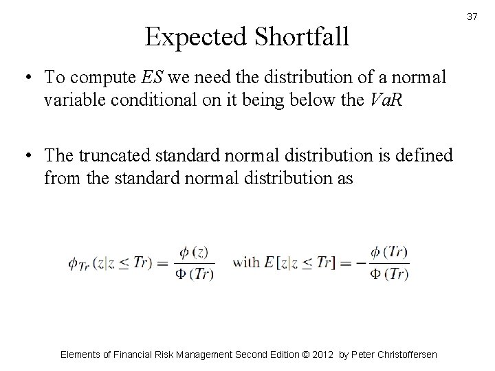
Expected Shortfall • To compute ES we need the distribution of a normal variable conditional on it being below the Va. R • The truncated standard normal distribution is defined from the standard normal distribution as Elements of Financial Risk Management Second Edition © 2012 by Peter Christoffersen 37

Expected Shortfall • ( ) denotes the density function and ( ) the cumulative density function of the standard normal distribution • In the normal distribution case ES can be derived as Elements of Financial Risk Management Second Edition © 2012 by Peter Christoffersen 38

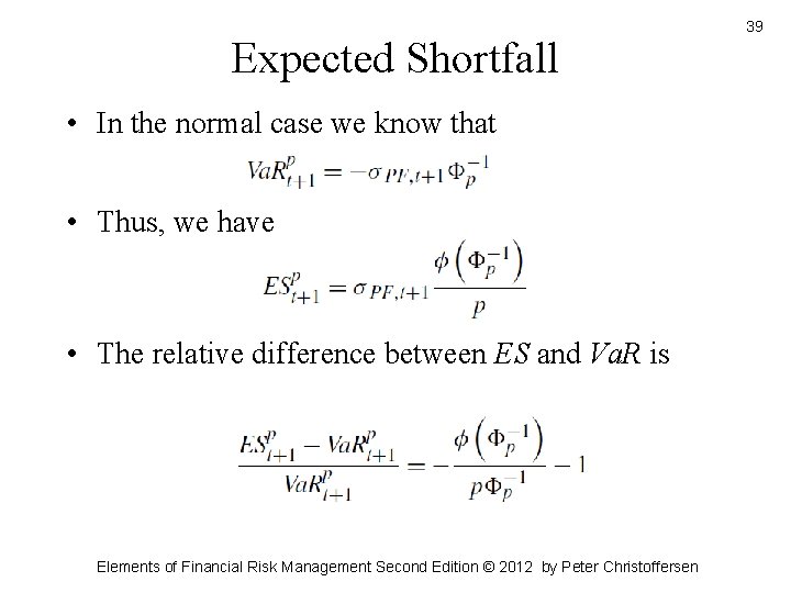
Expected Shortfall • In the normal case we know that • Thus, we have • The relative difference between ES and Va. R is Elements of Financial Risk Management Second Edition © 2012 by Peter Christoffersen 39

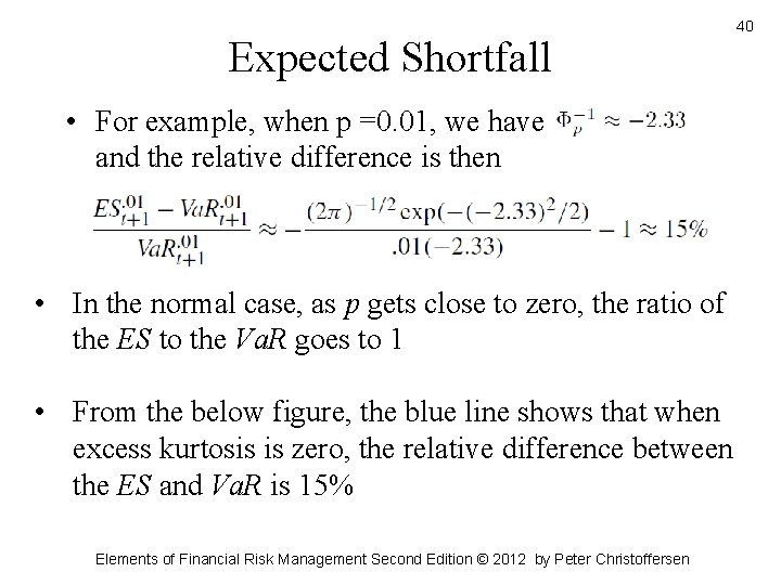
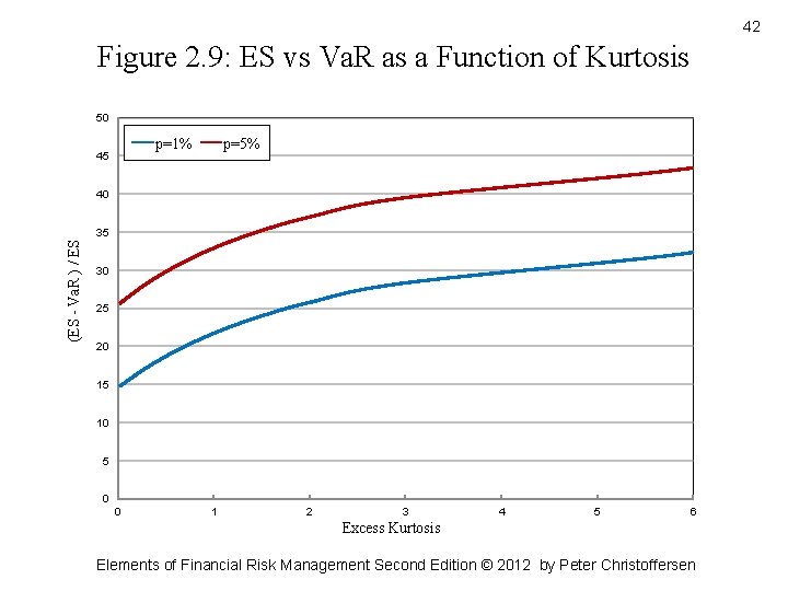
Expected Shortfall • For example, when p =0. 01, we have and the relative difference is then • In the normal case, as p gets close to zero, the ratio of the ES to the Va. R goes to 1 • From the below figure, the blue line shows that when excess kurtosis is zero, the relative difference between the ES and Va. R is 15% Elements of Financial Risk Management Second Edition © 2012 by Peter Christoffersen 40

Expected Shortfall • The blue line also shows that for moderately large values of excess kurtosis, the relative difference between ES and Va. R is above 30% • From the figure, the relative difference between Va. R and ES is larger when p is larger and thus further from zero • When p is close to zero Va. R and ES will both capture the fat tails in the distribution • When p is far from zero, only the ES will capture the fat tails in the return distribution Elements of Financial Risk Management Second Edition © 2012 by Peter Christoffersen 41

42 Figure 2. 9: ES vs Va. R as a Function of Kurtosis 50 p=1% 45 p=5% 40 (ES - Va. R ) / ES 35 30 25 20 15 10 5 0 0 1 2 3 4 5 6 Excess Kurtosis Elements of Financial Risk Management Second Edition © 2012 by Peter Christoffersen

Summary • Va. R is the most popular risk measure in use • HS is the most often used methodology to compute Va. R • Va. R has some shortcomings and using HS to compute Va. R has serious problems as well • We need to use risk measures that capture the degree of fatness in the tail of the return distribution • We need risk models that properly account for the dynamics in variance and models that can be used across different return horizons Elements of Financial Risk Management Second Edition © 2012 by Peter Christoffersen 43