1 Guidance on Intensity Guidance Kieran Bhatia David

1 Guidance on Intensity Guidance Kieran Bhatia, David Nolan, Mark De. Maria, Andrea Schumacher This project is supported by the NOAA Joint Hurricane Testbed. IHC Presentation 03 -03 -2015

2 Project Outline • Real-time guidance of intensity forecast error • Applications of error predictions

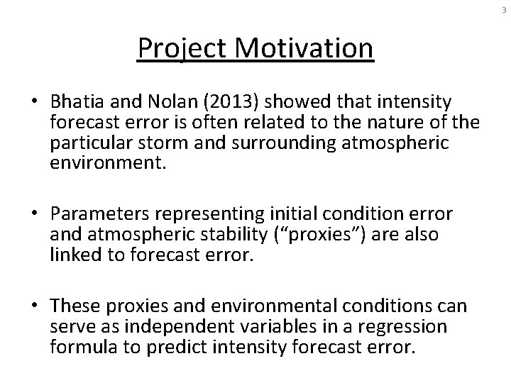
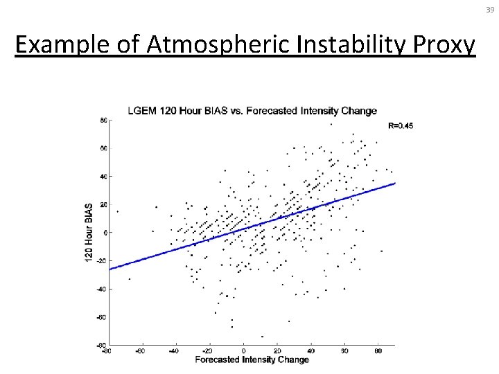
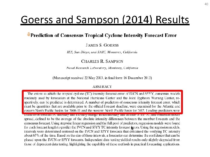
3 Project Motivation • Bhatia and Nolan (2013) showed that intensity forecast error is often related to the nature of the particular storm and surrounding atmospheric environment. • Parameters representing initial condition error and atmospheric stability (“proxies”) are also linked to forecast error. • These proxies and environmental conditions can serve as independent variables in a regression formula to predict intensity forecast error.

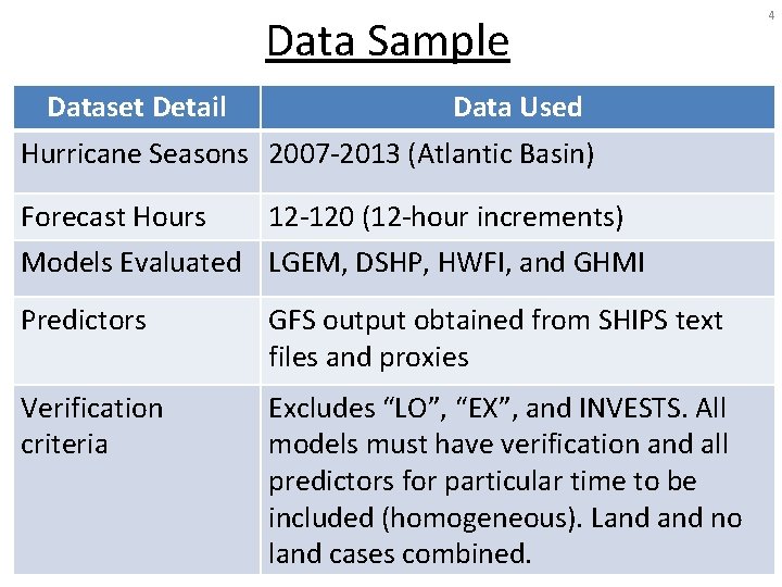
Data Sample Dataset Detail Data Used Hurricane Seasons 2007 -2013 (Atlantic Basin) Forecast Hours 12 -120 (12 -hour increments) Models Evaluated LGEM, DSHP, HWFI, and GHMI Predictors GFS output obtained from SHIPS text files and proxies Verification criteria Excludes “LO”, “EX”, and INVESTS. All models must have verification and all predictors for particular time to be included (homogeneous). Land no land cases combined. 4

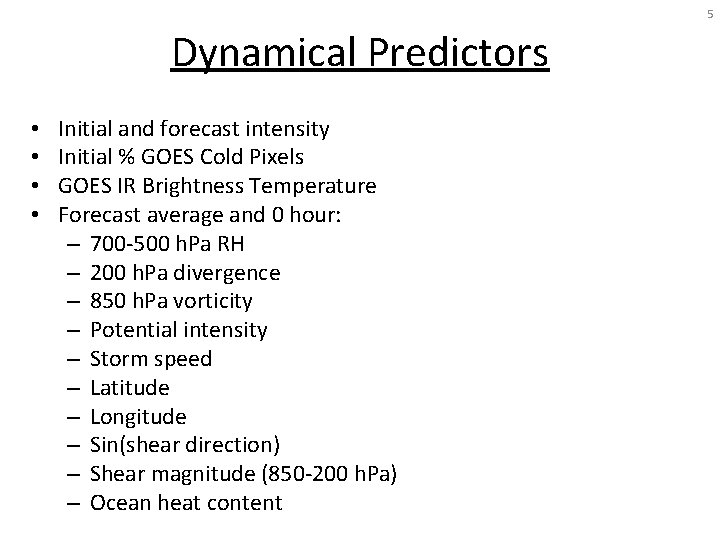
5 Dynamical Predictors • • Initial and forecast intensity Initial % GOES Cold Pixels GOES IR Brightness Temperature Forecast average and 0 hour: – 700 -500 h. Pa RH – 200 h. Pa divergence – 850 h. Pa vorticity – Potential intensity – Storm speed – Latitude – Longitude – Sin(shear direction) – Shear magnitude (850 -200 h. Pa) – Ocean heat content

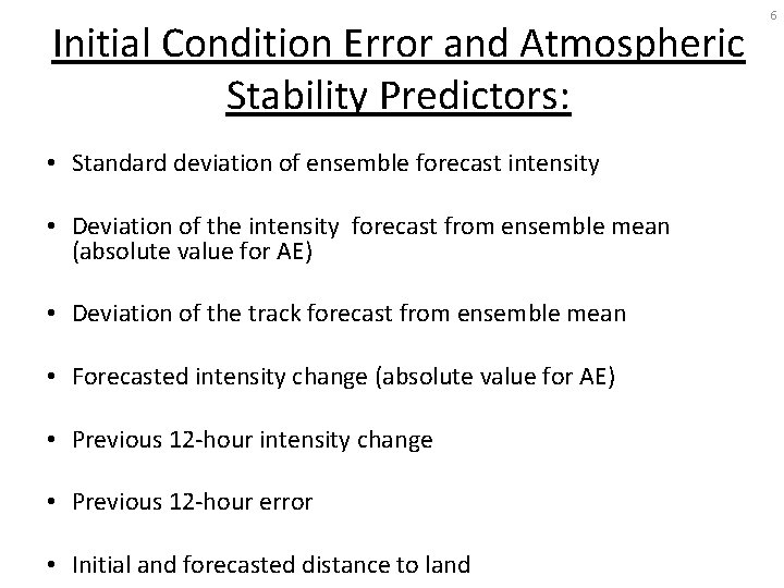
Initial Condition Error and Atmospheric Stability Predictors: • Standard deviation of ensemble forecast intensity • Deviation of the intensity forecast from ensemble mean (absolute value for AE) • Deviation of the track forecast from ensemble mean • Forecasted intensity change (absolute value for AE) • Previous 12 -hour intensity change • Previous 12 -hour error • Initial and forecasted distance to land 6

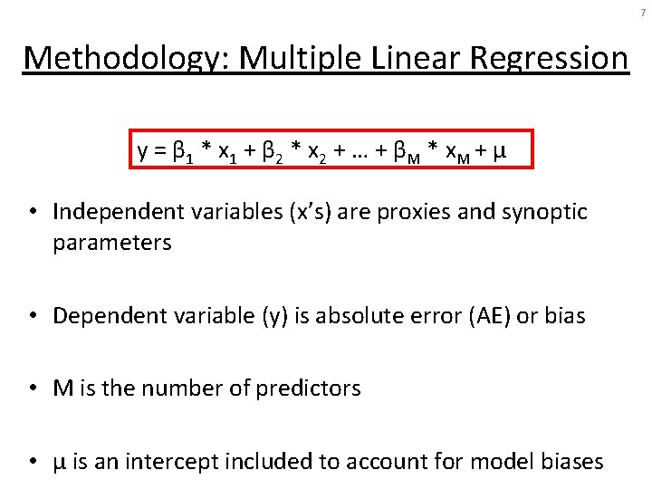
7 Methodology: Multiple Linear Regression y = β 1 * x 1 + β 2 * x 2 + … + βM * x. M + μ • Independent variables (x’s) are proxies and synoptic parameters • Dependent variable (y) is absolute error (AE) or bias • M is the number of predictors • μ is an intercept included to account for model biases

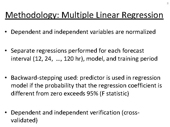
8 Methodology: Multiple Linear Regression • Dependent and independent variables are normalized • Separate regressions performed for each forecast interval (12, 24, …, 120 hr), model, and training period • Backward-stepping used: predictor is used in regression model if the probability that the regression coefficient is different from zero exceeds 95% (F statistic) • Dependent and independent verification (crossvalidated)

Predictor and Predictand Transformations • AE is bounded by 0, which leads to a positively skewed distribution • Box-Cox transformation applied to AE to make it approximately Gaussian before regression is applied • To account for non-linear relationships between predictors and forecast error, low order polynomials and Gaussian functions are applied to the predictors and tested • For example, 0 -hour relative humidity (RH) is fitted using a Gaussian to account for peak error at medium RH values 9

10 Results ALL RESULTS FOR INDEPENDENT DATASET, CROSS VALIDATION USED FOR 2007 -2014

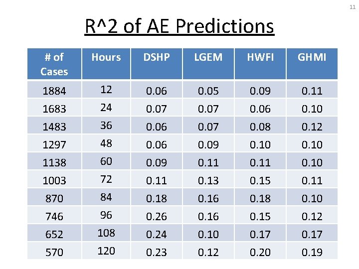
11 R^2 of AE Predictions # of Cases Hours DSHP LGEM HWFI GHMI 1884 12 24 0. 06 0. 05 0. 09 0. 11 0. 07 0. 06 0. 09 0. 11 0. 18 0. 26 0. 24 0. 07 0. 09 0. 11 0. 13 0. 16 0. 10 0. 06 0. 08 0. 10 0. 11 0. 15 0. 18 0. 15 0. 17 0. 10 0. 12 0. 10 0. 11 0. 10 0. 12 0. 17 0. 23 0. 12 0. 20 0. 19 1683 1483 1297 1138 1003 870 746 652 570 36 48 60 72 84 96 108 120

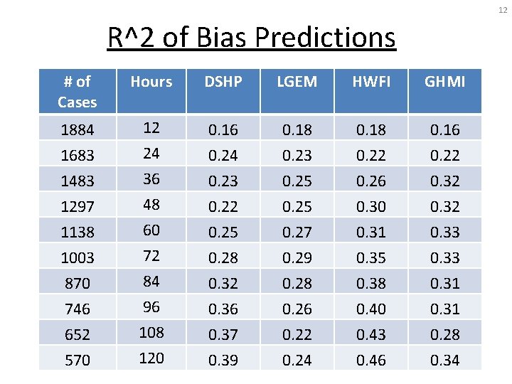
12 R^2 of Bias Predictions # of Cases Hours DSHP LGEM HWFI GHMI 1884 12 24 0. 16 0. 18 0. 16 0. 24 0. 23 0. 22 0. 25 0. 28 0. 32 0. 36 0. 37 0. 23 0. 25 0. 27 0. 29 0. 28 0. 26 0. 22 0. 26 0. 30 0. 31 0. 35 0. 38 0. 40 0. 43 0. 22 0. 32 0. 33 0. 31 0. 28 0. 39 0. 24 0. 46 0. 34 1683 1483 1297 1138 1003 870 746 652 570 36 48 60 72 84 96 108 120

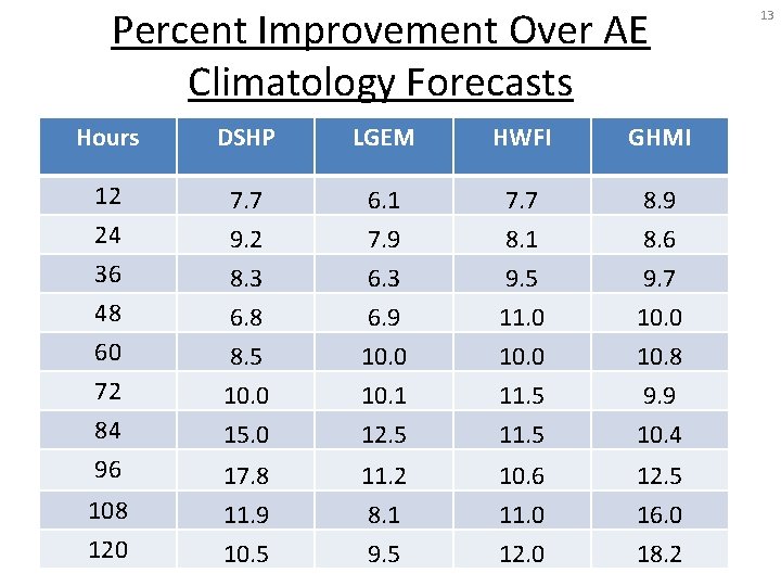
Percent Improvement Over AE Climatology Forecasts Hours DSHP LGEM HWFI GHMI 12 24 7. 7 6. 1 7. 7 8. 9 9. 2 8. 3 6. 8 8. 5 10. 0 15. 0 7. 9 6. 3 6. 9 10. 0 10. 1 12. 5 8. 1 9. 5 11. 0 10. 0 11. 5 8. 6 9. 7 10. 0 10. 8 9. 9 10. 4 17. 8 11. 9 11. 2 8. 1 10. 6 11. 0 12. 5 16. 0 10. 5 9. 5 12. 0 18. 2 36 48 60 72 84 96 108 120 13

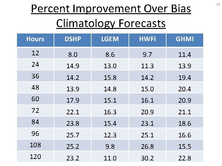
Percent Improvement Over Bias Climatology Forecasts Hours DSHP LGEM HWFI GHMI 12 8. 0 8. 6 9. 7 11. 4 24 14. 9 13. 0 11. 3 13. 9 36 14. 2 15. 8 14. 2 19. 4 48 13. 9 14. 8 15. 0 20. 4 60 17. 9 15. 1 16. 1 20. 9 72 22. 1 16. 3 20. 9 21. 1 84 23. 8 15. 4 23. 1 18. 6 96 25. 7 12. 3 25. 1 16. 6 108 25. 2 9. 8 26. 8 15. 5 120 23. 2 11. 0 30. 2 22. 8 14

15 Applications

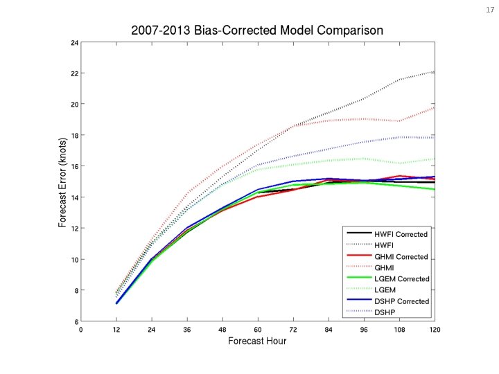
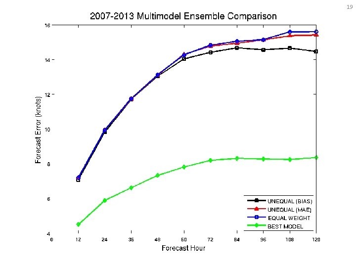
16 Motivation • If model error can be successfully anticipated in certain situations, can we bias-correct the models or weight an ensemble accordingly? • Two first attempts to create unequally weighted ensembles can be derived from AE and bias predictions.

17

Methodology For Unequally Weighted Ensemble • Technique 1 – Bias-correct individual models using bias forecasts and use the mean of the bias-corrected models • Technique 2 – Inverse-weight individual models using AE forecasts and use the inverse-weighted average as the ensemble mean – i. e. if LGEM is predicted to have 20 knots of AE and DSHP is predicted to have 10 knots of AE, trust DSHP’s forecast more 18

19

20 Conclusions • Predictor pool selected using results of Bhatia and Nolan (2013) and added proxies • Inputted into a modified multiple linear regression model • Multiple linear regression techniques are promising with 2007 -2014 independent results showing percent improvement over climatology ranging from 6%-18% for AE and 8%-30% for bias

21 Extra Slides

22 Future Work • Testing more proxies • Developing nonlinear relationships between predictors and forecast error • Varying the length of training period • Producing error predictions using probabilistic forecasts • Neural networking and nonlinear regression methods may be considered

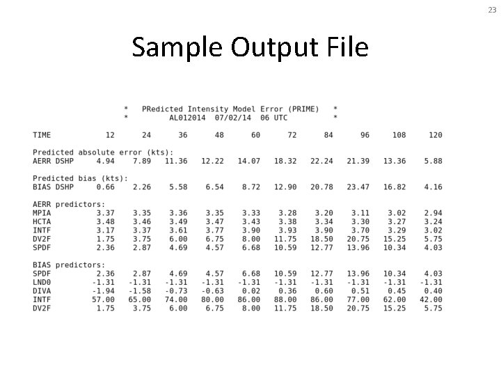
23 Sample Output File

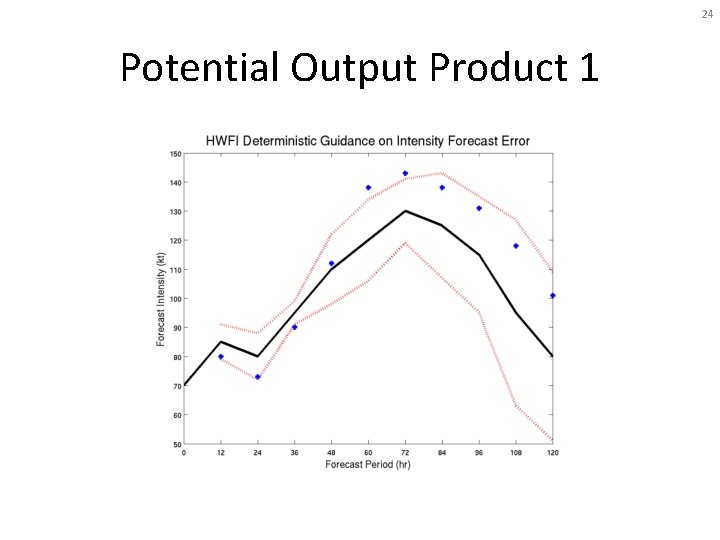
24 Potential Output Product 1

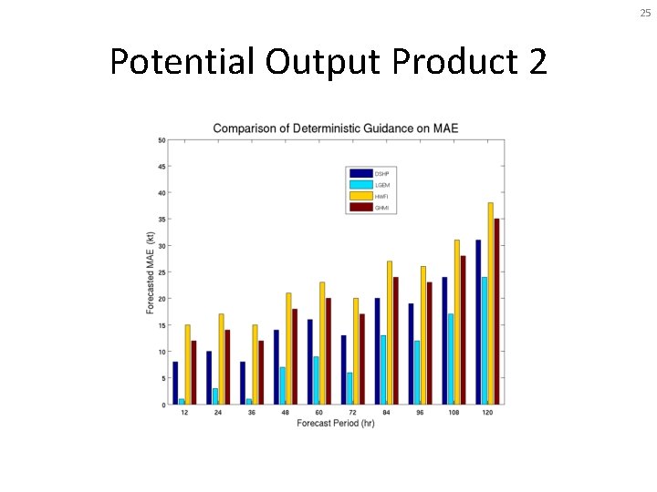
25 Potential Output Product 2

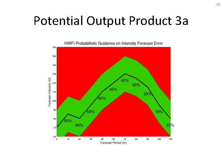
26 Potential Output Product 3 a

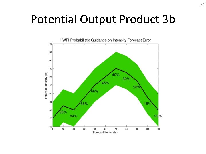
27 Potential Output Product 3 b

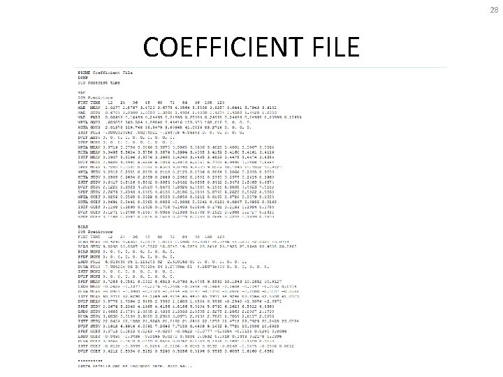
28 COEFFICIENT FILE

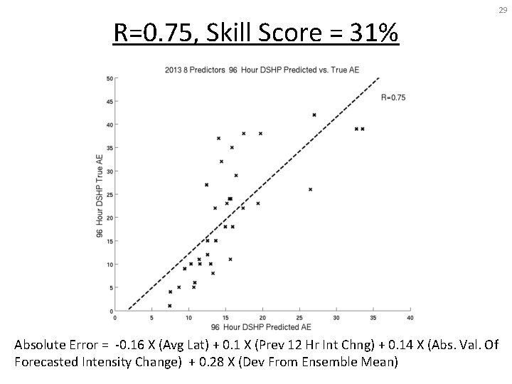
R=0. 75, Skill Score = 31% Absolute Error = -0. 16 X (Avg Lat) + 0. 1 X (Prev 12 Hr Int Chng) + 0. 14 X (Abs. Val. Of Forecasted Intensity Change) + 0. 28 X (Dev From Ensemble Mean) 29

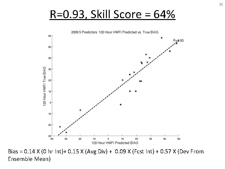
R=0. 93, Skill Score = 64% Bias = 0. 14 X (0 hr Int)+ 0. 15 X (Avg Div) + 0. 09 X (Fcst Int) + 0. 57 X (Dev From Ensemble Mean) 30

31 Probabilistic Forecasts of AE and Bias

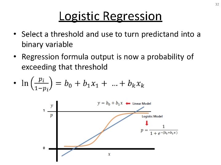
32 Logistic Regression •

33 Methodology: Probabilistic Forecasts • AE and Bias were converted to binary and ternary variables • AE: Binary threshold = 20 knots, Ternary thresholds= 10 knots and 20 knots • Bias: Binary threshold = 0 knots, Ternary thresholds= -20 knots and 20 knots

34 Reliability Diagram • Graphical device that shows the full joint distribution of the forecasts and observations • Observed frequency of an event is plotted against the forecast probability of an event • A perfect forecast system will result in forecasts with a probability of X% actually occurring X% of the time (diagonal line on the graph)

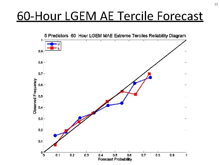
35 60 -Hour LGEM AE Tercile Forecast

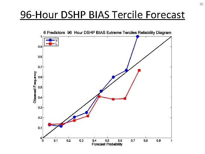
36 96 -Hour DSHP BIAS Tercile Forecast

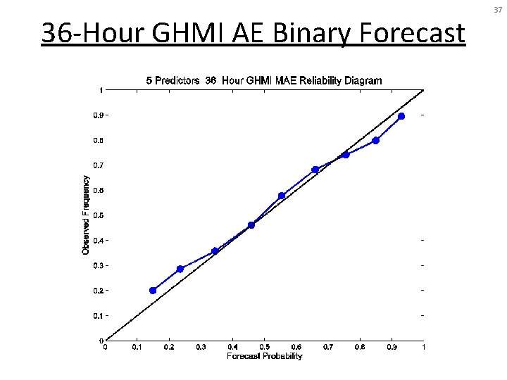
36 -Hour GHMI AE Binary Forecast 37

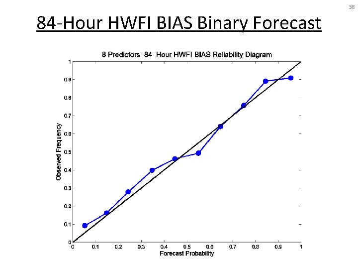
84 -Hour HWFI BIAS Binary Forecast 38

39 Example of Atmospheric Instability Proxy

40 Goerss and Sampson (2014) Results

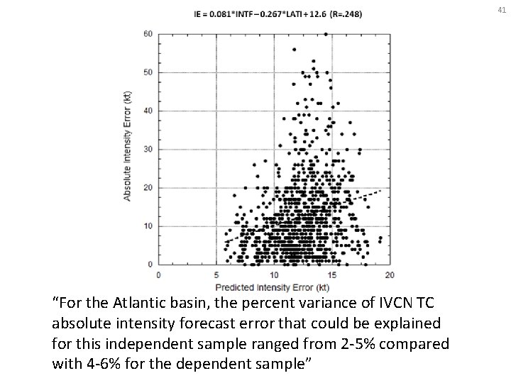
41 “For the Atlantic basin, the percent variance of IVCN TC absolute intensity forecast error that could be explained for this independent sample ranged from 2 -5% compared with 4 -6% for the dependent sample”

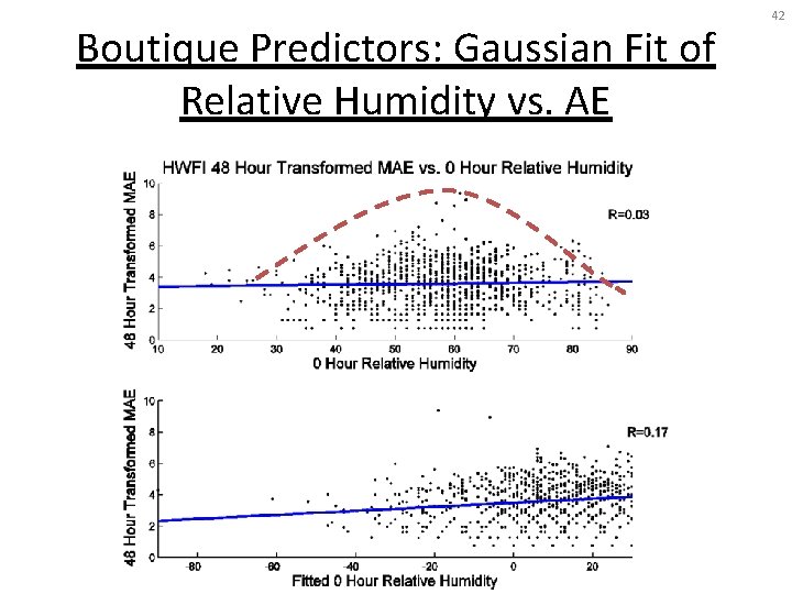
Boutique Predictors: Gaussian Fit of Relative Humidity vs. AE 42

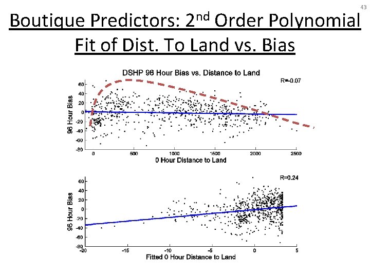
43 Boutique Predictors: 2 nd Order Polynomial Fit of Dist. To Land vs. Bias

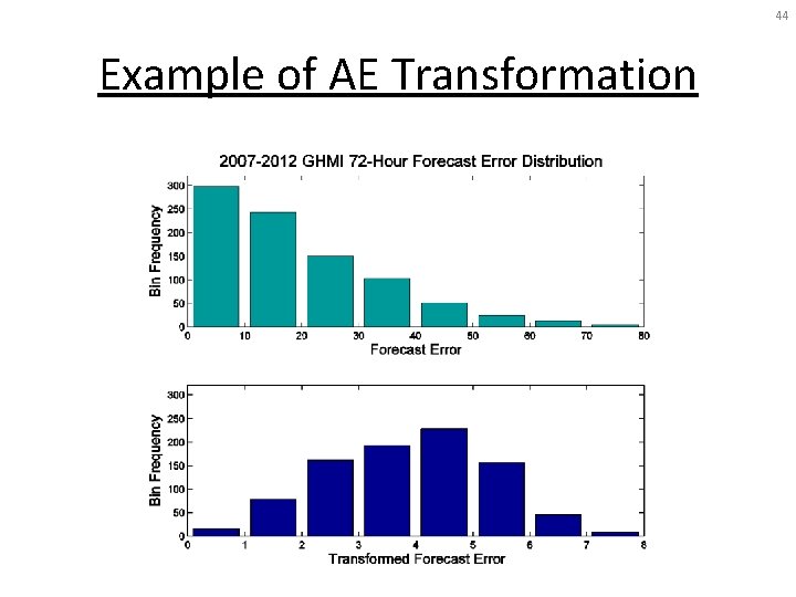
44 Example of AE Transformation

Methodology: Nonlinear Fits of Predictors • Several predictors exhibiting nonlinear relationships with error were empirically fit • Functions tested: Gaussian, second order polynomial, and third order polynomial • 0 -Hour Latitude, 0 -Hour distance to land, and 0 -Hour Relative Humidity exhibited the strongest non-linear relationships 45

46 2014 RESULTS

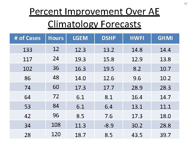
47 Percent Improvement Over AE Climatology Forecasts # of Cases Hours LGEM DSHP HWFI GHMI 133 117 102 86 74 64 12 24 36 48 60 72 12. 3 19. 3 16. 3 14. 0 17. 3 6. 1 13. 2 15. 8 19. 5 12. 6 17. 7 8. 1 14. 8 12. 9 8. 2 9. 6 28. 9 16. 4 14. 4 13. 8 10. 7 10. 2 28. 3 14. 7 53 42 34 28 84 96 108 6. 1 8. 5 11. 3 18. 7 6. 4 7. 6 -8. 9 8. 5 13. 1 17. 3 30. 2 43. 5 11. 1 18. 0 28. 8 39. 7 120

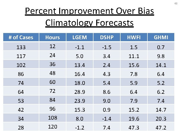
48 Percent Improvement Over Bias Climatology Forecasts # of Cases 133 117 102 86 74 64 53 42 34 28 Hours 12 24 36 48 60 72 84 96 108 120 LGEM DSHP HWFI GHMI -1. 1 5. 0 13. 4 16. 4 18. 0 28. 9 23. 9 15. 3 8. 0 -1. 2 -1. 5 3. 4 2. 4 4. 3 5. 4 8. 6 9. 0 0. 9 -1. 4 7. 4 1. 5 11. 1 15. 6 7. 8 5. 9 6. 4 7. 9 15. 2 19. 6 47. 3 0. 7 9. 8 14. 1 6. 4 5. 2 6. 2 7. 4 14. 7 20. 3 47. 2