1 DSP Processors Finite Impulse Response Filters 2

1

پﺮﺩﺍﺯﺷگﺮﻫﺎی ﺳیگﻨﺎﻟﻬﺎی ﺩیﺠیﺘﺎﻝ DSP Processors Finite Impulse Response Filters 2

Outlines �Introduction to the z- transform �Design and implementation of finite impulse response (FIR) filters �Programming examples using C and TMS 320 C 6 x code 3

INTRODUCTION TO THE z-TRANSFORM �Z-Transform Analyzing discrete-time signals �Laplace Transform Analyzing continuous-time signals �Analog filter Differential equation �Laplace transform for solving differential equations �Digital filter Difference equation �Z-transform for solving Difference equation 4

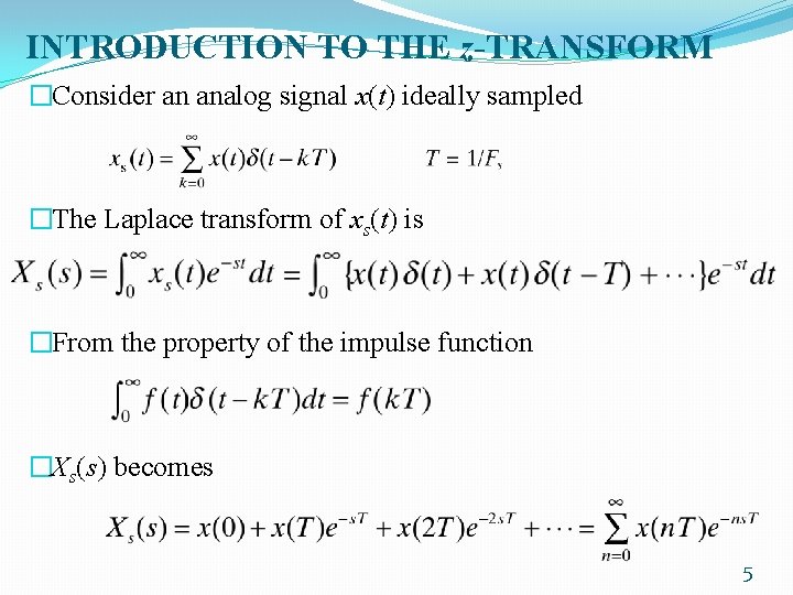
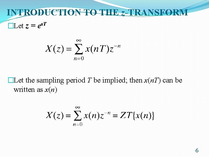
INTRODUCTION TO THE z-TRANSFORM �Consider an analog signal x(t) ideally sampled �The Laplace transform of xs(t) is �From the property of the impulse function �Xs(s) becomes 5

INTRODUCTION TO THE z-TRANSFORM �Let z = es. T �Let the sampling period T be implied; then x(n. T) can be written as x(n) 6

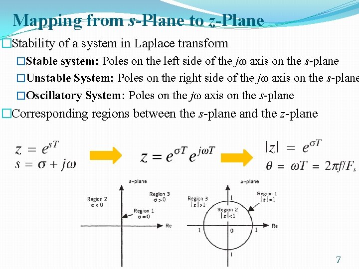
Mapping from s-Plane to z-Plane �Stability of a system in Laplace transform �Stable system: Poles on the left side of the jω axis on the s-plane �Unstable System: Poles on the right side of the jω axis on the s-plane �Oscillatory System: Poles on the jω axis on the s-plane �Corresponding regions between the s-plane and the z-plane 7

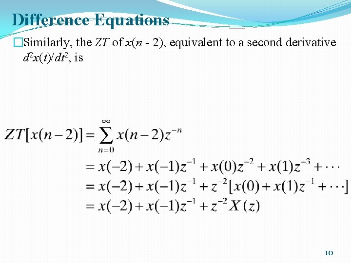
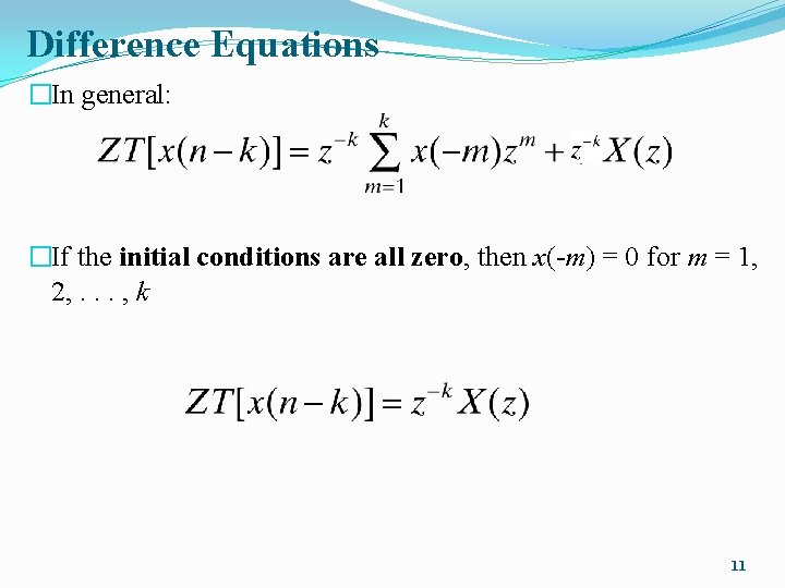
Difference Equations �Analog filter differential equation. �Digital filter difference equation. �To solve a difference equation: �we need to find the z- transform of expressions such as x(n - k), which corresponds to the kth derivative dk x(t)/dtk of an analog signal x(t). �The order of the difference equation is determined by the largest value of k. 8

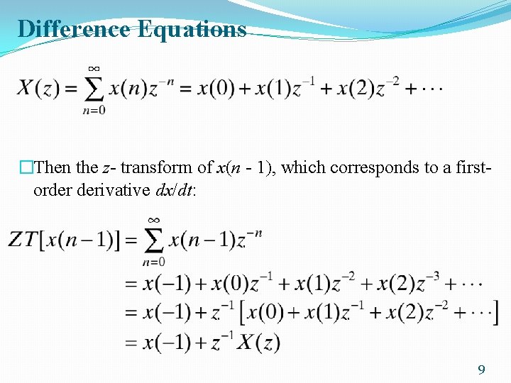
Difference Equations �Then the z- transform of x(n - 1), which corresponds to a firstorder derivative dx/dt: 9

Difference Equations �Similarly, the ZT of x(n - 2), equivalent to a second derivative d 2 x(t)/dt 2, is 10

Difference Equations �In general: �If the initial conditions are all zero, then x(-m) = 0 for m = 1, 2, . . . , k 11

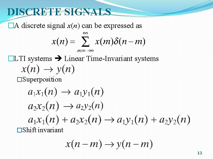
DISCRETE SIGNALS �A discrete signal x(n) can be expressed as �LTI systems Linear Time-Invariant systems �Superposition �Shift invariant 12

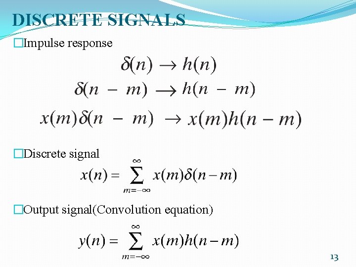
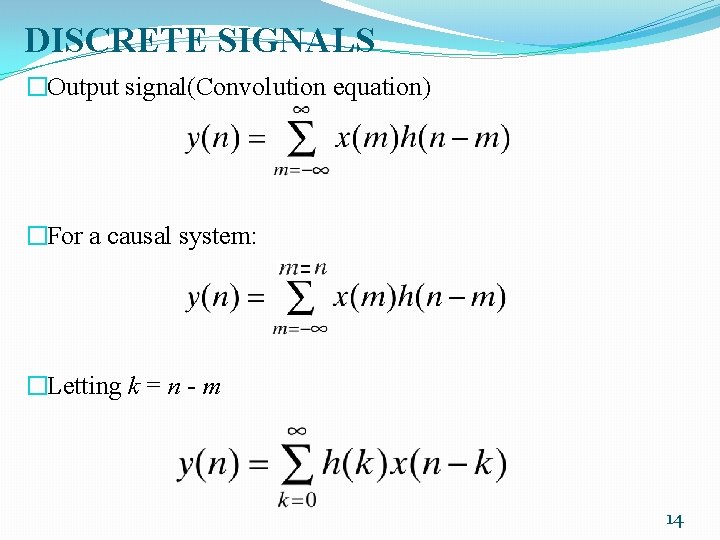
DISCRETE SIGNALS �Impulse response �Discrete signal �Output signal(Convolution equation) 13

DISCRETE SIGNALS �Output signal(Convolution equation) �For a causal system: �Letting k = n - m 14

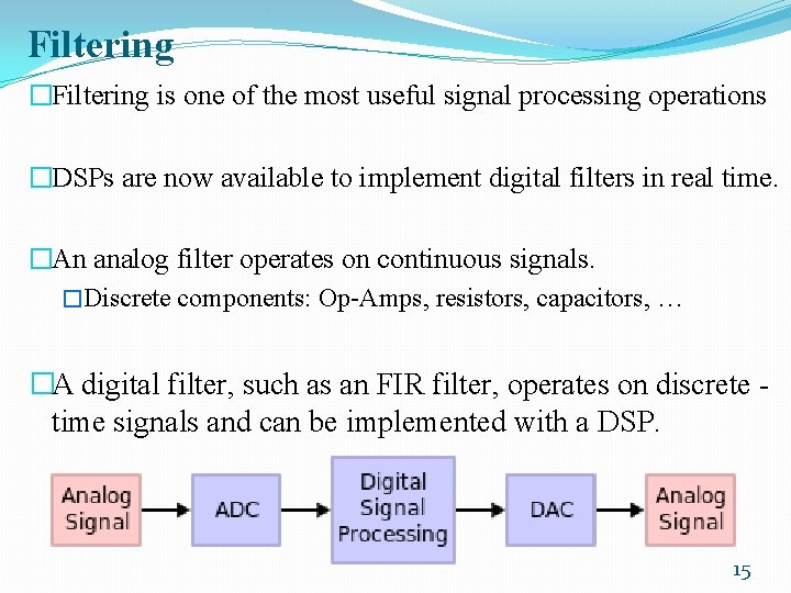
Filtering �Filtering is one of the most useful signal processing operations �DSPs are now available to implement digital filters in real time. �An analog filter operates on continuous signals. �Discrete components: Op-Amps, resistors, capacitors, … �A digital filter, such as an FIR filter, operates on discrete time signals and can be implemented with a DSP. 15

Digital filters �Digital filters have numerous advantages over their analog counterparts �The cost of DSPs has been reduced significantly �The processing power of DSPs has been enhanced significantly �Higher reliability, �Higher accuracy, �Less sensitivity to temperature and aging �Precise magnitude and phase characteristics can be achieved �Filter characteristics such as center frequency, bandwidth, and filter type can easily be modified. �A number of tools are available to design and implement within a few minutes an FIR filter in real time using the TMS 320 C 6 x based DSK. �…. 16

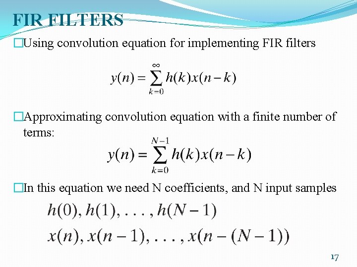
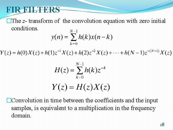
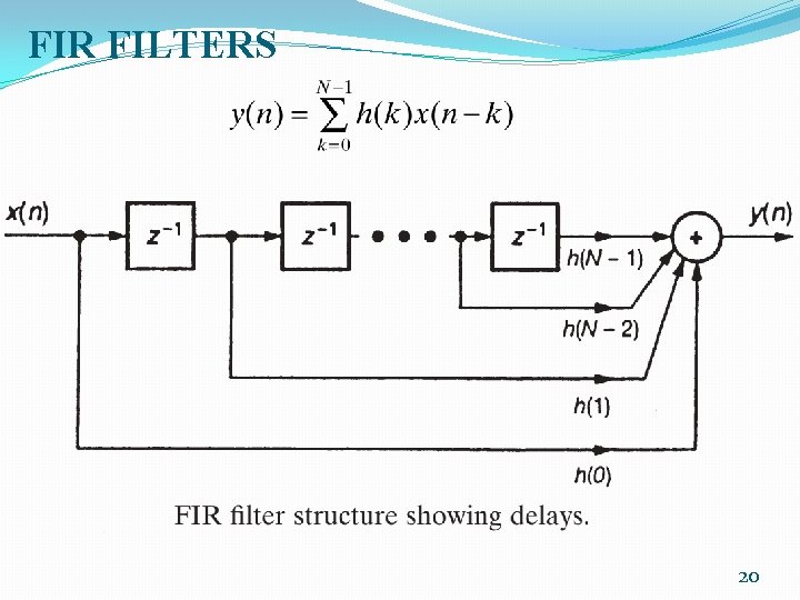
FIR FILTERS �Using convolution equation for implementing FIR filters �Approximating convolution equation with a finite number of terms: �In this equation we need N coefficients, and N input samples 17

FIR FILTERS �The z- transform of the convolution equation with zero initial conditions. �Convolution in time between the coefficients and the input samples, is equivalent to a multiplication in the frequency domain. 18

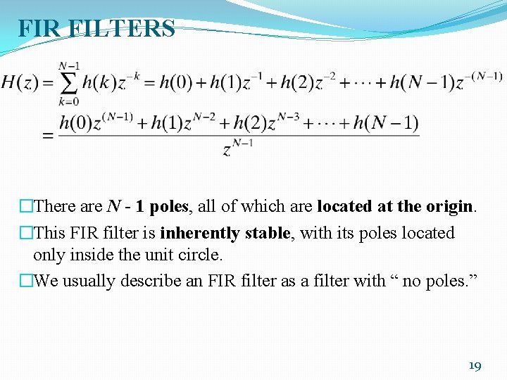
FIR FILTERS �There are N - 1 poles, all of which are located at the origin. �This FIR filter is inherently stable, with its poles located only inside the unit circle. �We usually describe an FIR filter as a filter with “ no poles. ” 19

FIR FILTERS 20

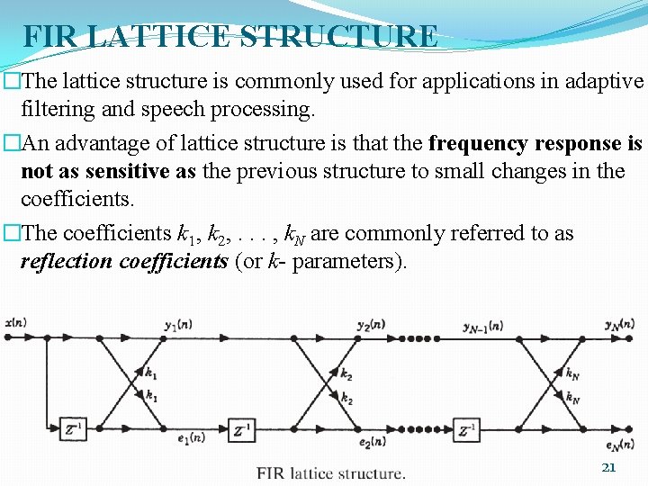
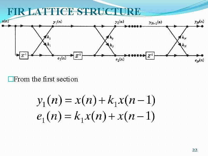
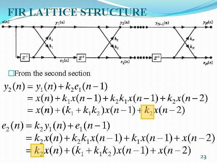
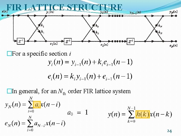
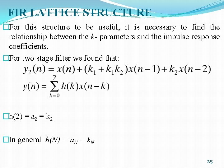
FIR LATTICE STRUCTURE �The lattice structure is commonly used for applications in adaptive filtering and speech processing. �An advantage of lattice structure is that the frequency response is not as sensitive as the previous structure to small changes in the coefficients. �The coefficients k 1, k 2, . . . , k. N are commonly referred to as reflection coefficients (or k- parameters). 21

FIR LATTICE STRUCTURE �From the first section 22

FIR LATTICE STRUCTURE �From the second section 23

FIR LATTICE STRUCTURE �For a specific section i �In general, for an Nth order FIR lattice system 24

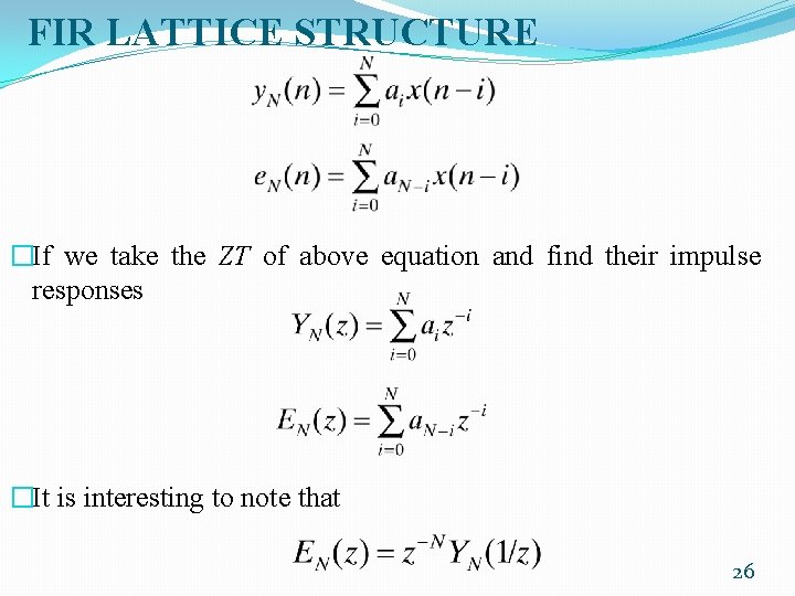
FIR LATTICE STRUCTURE �For this structure to be useful, it is necessary to find the relationship between the k- parameters and the impulse response coefficients. �For two stage filter we found that: �h(2) = a 2 = k 2 �In general h(N) = a. N = k. N 25

FIR LATTICE STRUCTURE �If we take the ZT of above equation and find their impulse responses �It is interesting to note that 26

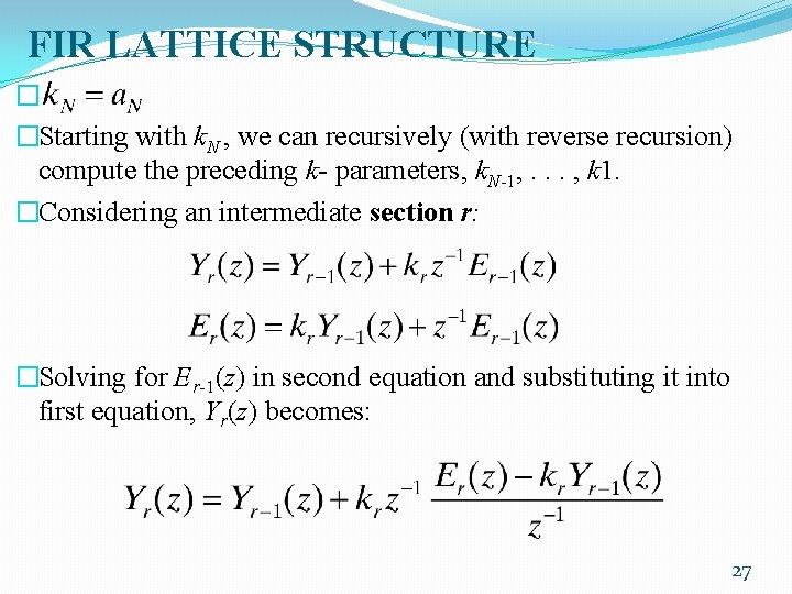
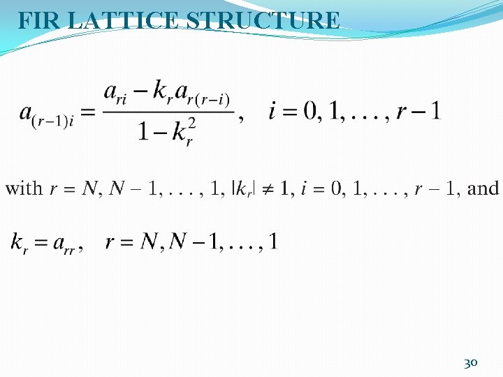
FIR LATTICE STRUCTURE � �Starting with k. N , we can recursively (with reverse recursion) compute the preceding k- parameters, k. N-1, . . . , k 1. �Considering an intermediate section r: �Solving for Er-1(z) in second equation and substituting it into first equation, Yr(z) becomes: 27

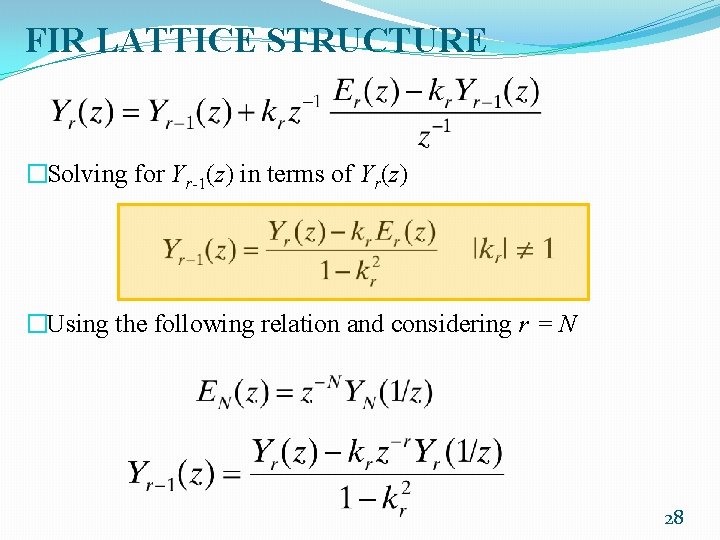
FIR LATTICE STRUCTURE �Solving for Yr-1(z) in terms of Yr(z) �Using the following relation and considering r = N 28

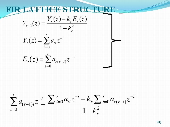
FIR LATTICE STRUCTURE 29

FIR LATTICE STRUCTURE 30

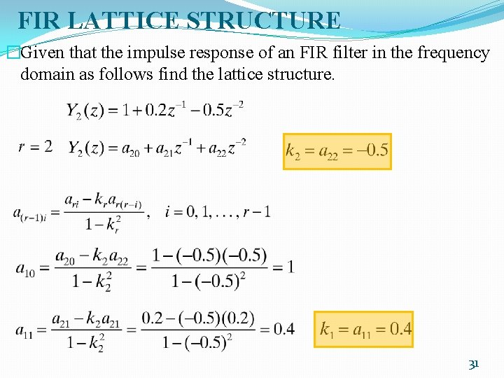
FIR LATTICE STRUCTURE �Given that the impulse response of an FIR filter in the frequency domain as follows find the lattice structure. 31

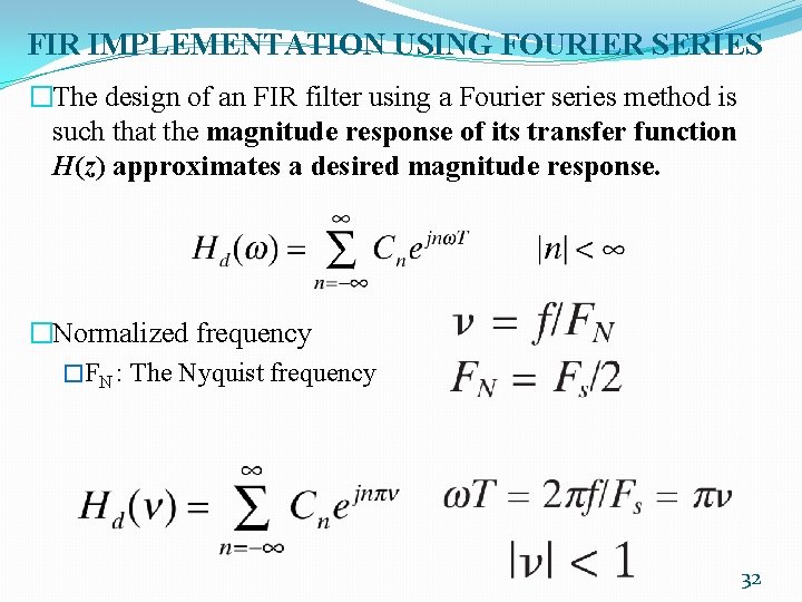
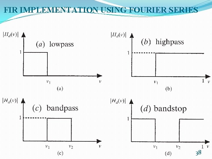
FIR IMPLEMENTATION USING FOURIER SERIES �The design of an FIR filter using a Fourier series method is such that the magnitude response of its transfer function H(z) approximates a desired magnitude response. �Normalized frequency �FN : The Nyquist frequency 32

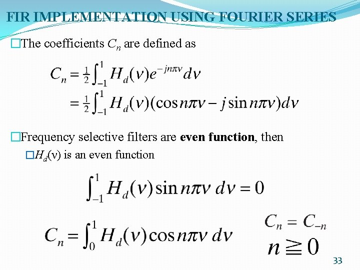
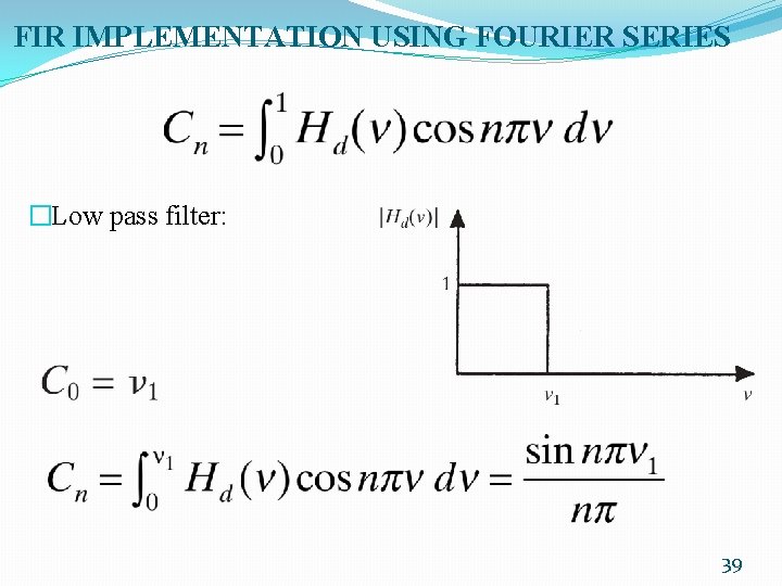
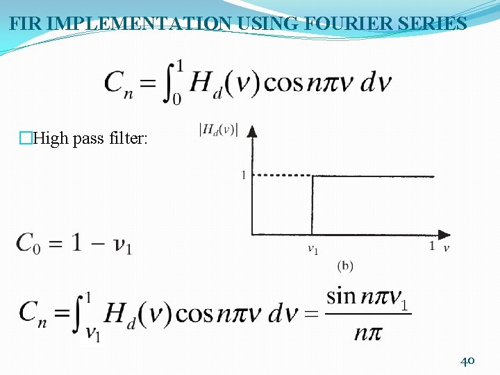
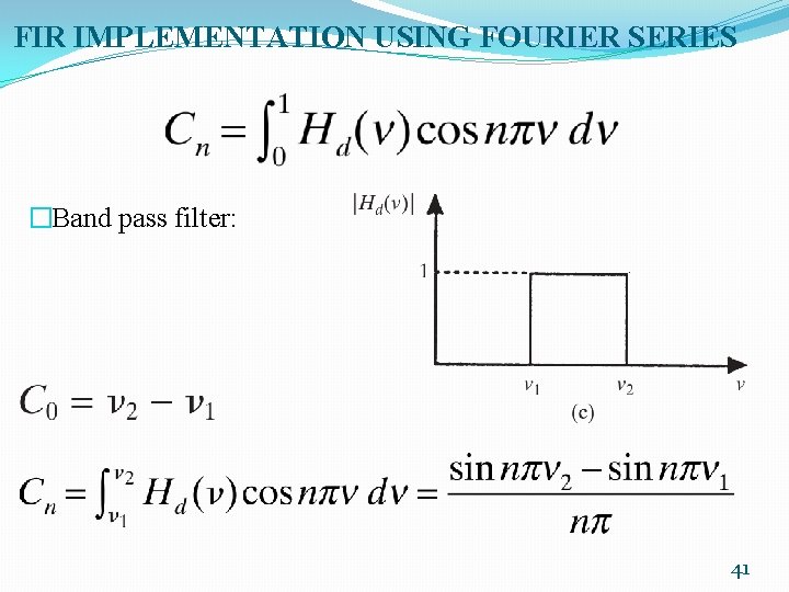
FIR IMPLEMENTATION USING FOURIER SERIES �The coefficients Cn are defined as �Frequency selective filters are even function, then �Hd(ν) is an even function 33

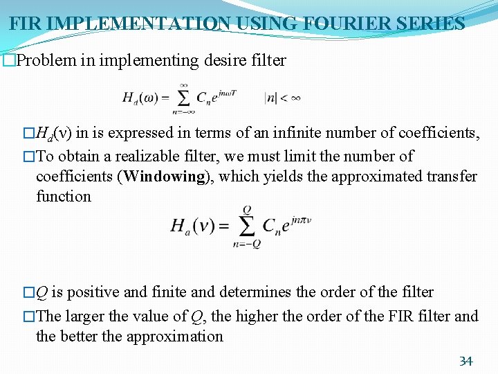
FIR IMPLEMENTATION USING FOURIER SERIES �Problem in implementing desire filter �Hd(ν) in is expressed in terms of an infinite number of coefficients, �To obtain a realizable filter, we must limit the number of coefficients (Windowing), which yields the approximated transfer function �Q is positive and finite and determines the order of the filter �The larger the value of Q, the higher the order of the FIR filter and the better the approximation 34

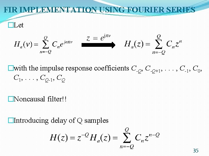
FIR IMPLEMENTATION USING FOURIER SERIES �Let �with the impulse response coefficients C-Q, C-Q+1, . . . , C-1, C 0, C 1, . . . , CQ-1, CQ �Noncausal filter!! �Introducing delay of Q samples 35

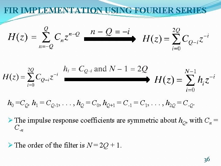
FIR IMPLEMENTATION USING FOURIER SERIES h 0 =CQ, h 1 = CQ-1, . . . , h. Q = C 0, h. Q+1 = C-1 = C 1, . . . , h 2 Q = C-Q. Ø The impulse response coefficients are symmetric about h. Q, with Cn = C-n Ø The order of the filter is N = 2 Q + 1. 36

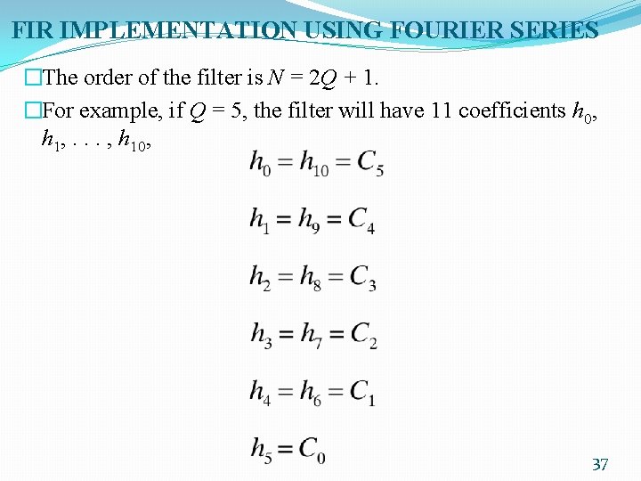
FIR IMPLEMENTATION USING FOURIER SERIES �The order of the filter is N = 2 Q + 1. �For example, if Q = 5, the filter will have 11 coefficients h 0, h 1, . . . , h 10, 37

FIR IMPLEMENTATION USING FOURIER SERIES 38

FIR IMPLEMENTATION USING FOURIER SERIES �Low pass filter: 39

FIR IMPLEMENTATION USING FOURIER SERIES �High pass filter: 40

FIR IMPLEMENTATION USING FOURIER SERIES �Band pass filter: 41

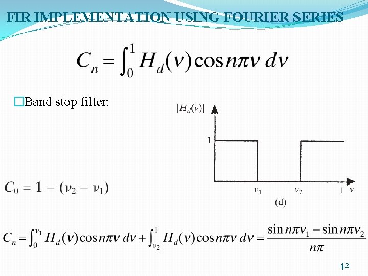
FIR IMPLEMENTATION USING FOURIER SERIES �Band stop filter: 42

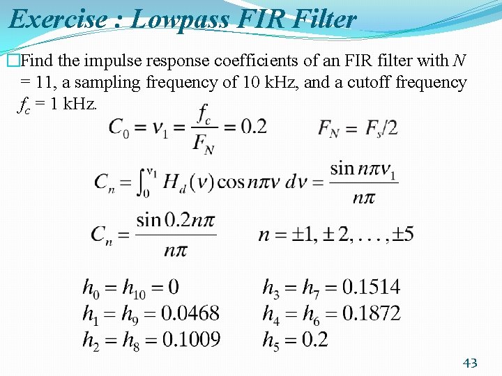
Exercise : Lowpass FIR Filter �Find the impulse response coefficients of an FIR filter with N = 11, a sampling frequency of 10 k. Hz, and a cutoff frequency fc = 1 k. Hz. 43

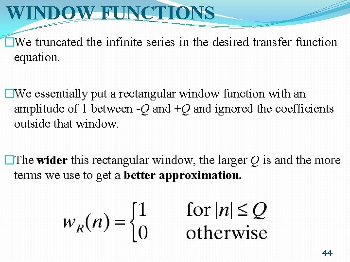
WINDOW FUNCTIONS �We truncated the infinite series in the desired transfer function equation. �We essentially put a rectangular window function with an amplitude of 1 between -Q and +Q and ignored the coefficients outside that window. �The wider this rectangular window, the larger Q is and the more terms we use to get a better approximation. 44

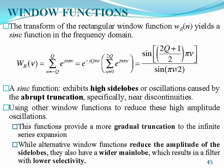
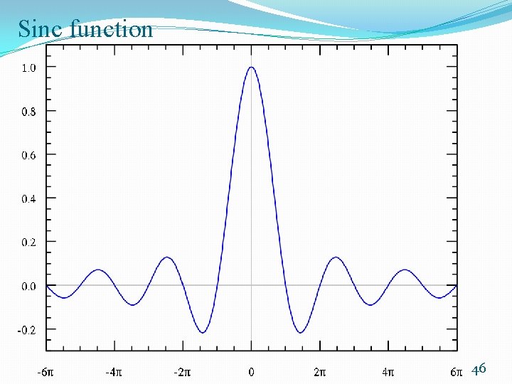
WINDOW FUNCTIONS �The transform of the rectangular window function w. R(n) yields a sinc function in the frequency domain. �A sinc function: exhibits high sidelobes or oscillations caused by the abrupt truncation, specifically, near discontinuities. �Using other window functions to reduce these high amplitude oscillations. �This functions provide a more gradual truncation to the infinite series expansion �While alternative window functions reduce the amplitude of the sidelobes, they also have a wider mainlobe, which results in a filter with lower selectivity. 45

Sinc function 46

WINDOW FUNCTIONS �A measure of a filter’s performance is a ripple factor that compares the peak of the first sidelobe to the peak of the mainlobe (their ratio). �A compromise or trade-off between �Selecting a window function that can reduce the sidelobes �Approaching the selectivity that can be achieved with the rectangular window function. �The width of the mainlobe can be reduced by increasing the width of the window (order of the filter). 47

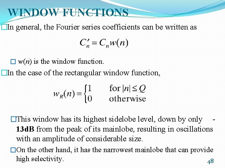
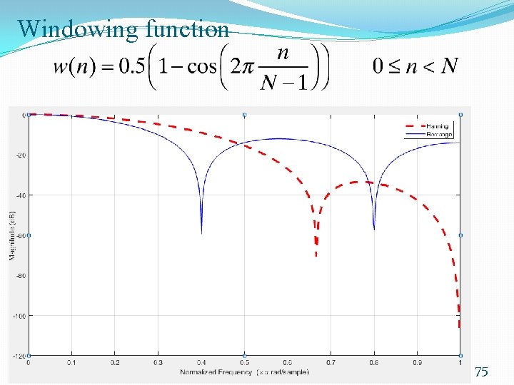
WINDOW FUNCTIONS �In general, the Fourier series coefficients can be written as � w(n) is the window function. �In the case of the rectangular window function, �This window has its highest sidelobe level, down by only 13 d. B from the peak of its mainlobe, resulting in oscillations with an amplitude of considerable size. �On the other hand, it has the narrowest mainlobe that can provide high selectivity. 48

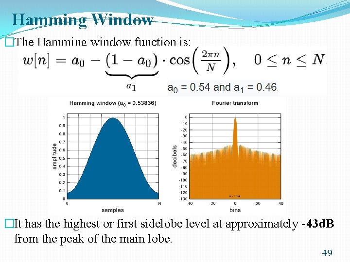
Hamming Window �The Hamming window function is: �It has the highest or first sidelobe level at approximately -43 d. B from the peak of the main lobe. 49

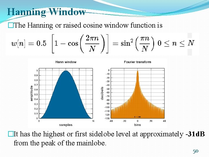
Hanning Window �The Hanning or raised cosine window function is �It has the highest or first sidelobe level at approximately -31 d. B from the peak of the mainlobe. 50

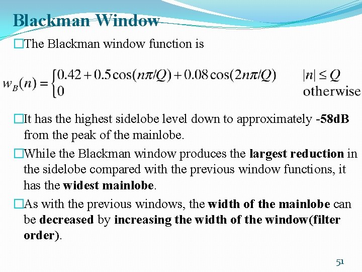
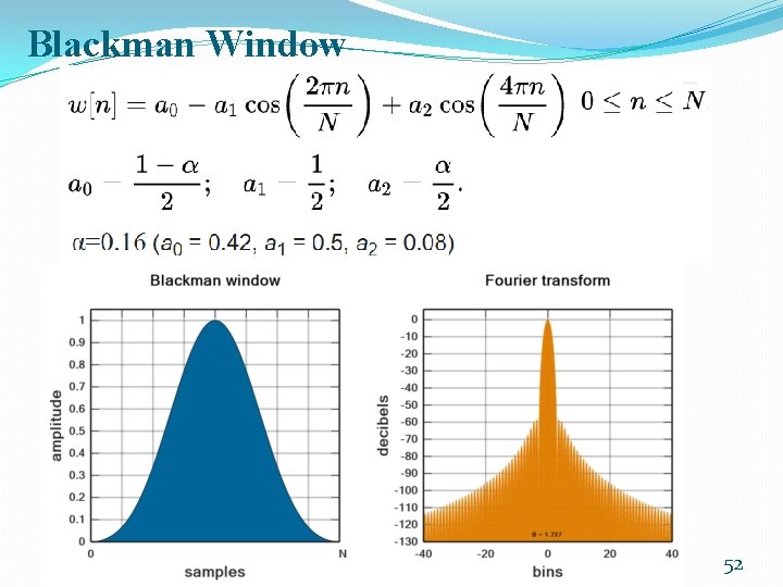
Blackman Window �The Blackman window function is �It has the highest sidelobe level down to approximately -58 d. B from the peak of the mainlobe. �While the Blackman window produces the largest reduction in the sidelobe compared with the previous window functions, it has the widest mainlobe. �As with the previous windows, the width of the mainlobe can be decreased by increasing the width of the window(filter order). 51

Blackman Window 52

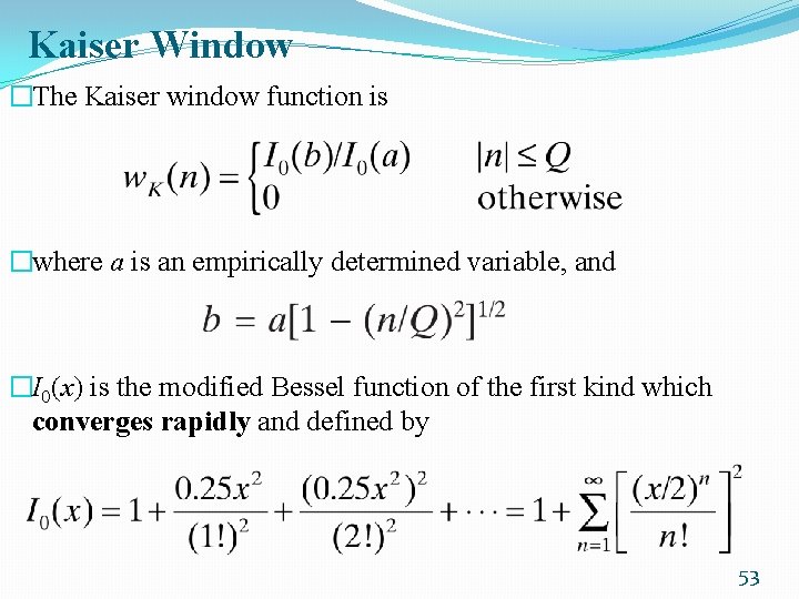
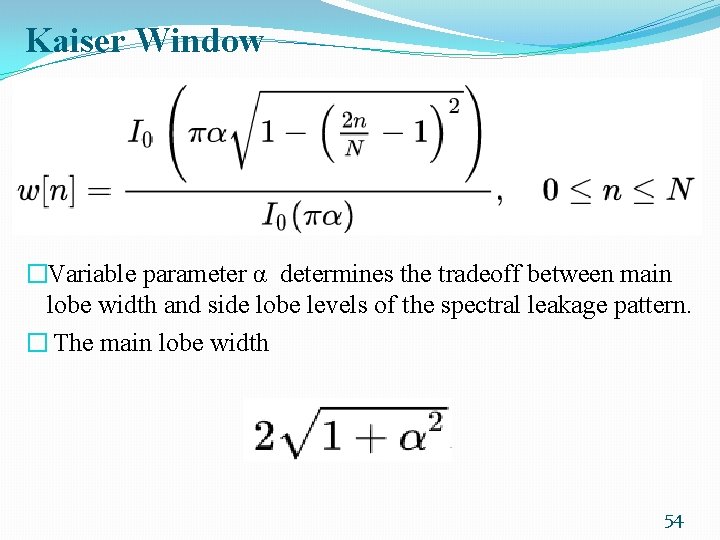
Kaiser Window �The Kaiser window function is �where a is an empirically determined variable, and �I 0(x) is the modified Bessel function of the first kind which converges rapidly and defined by 53

Kaiser Window �Variable parameter α determines the tradeoff between main lobe width and side lobe levels of the spectral leakage pattern. � The main lobe width 54

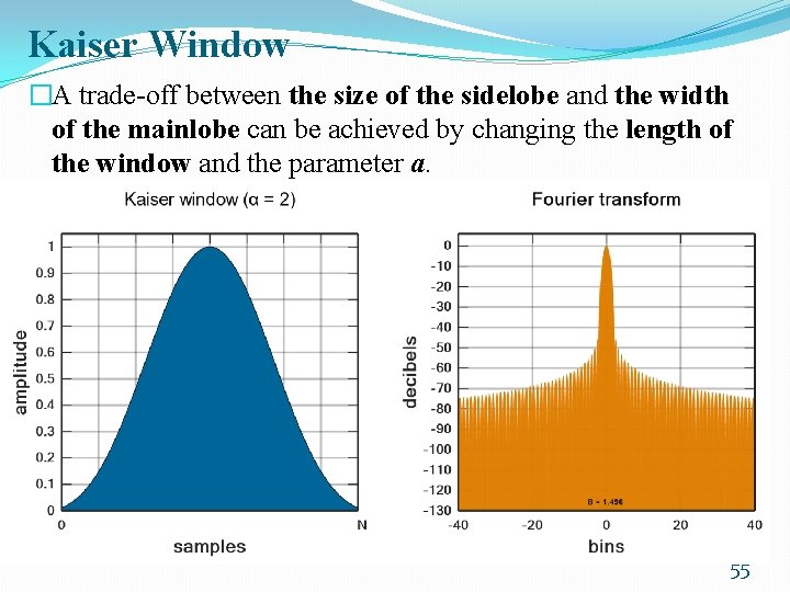
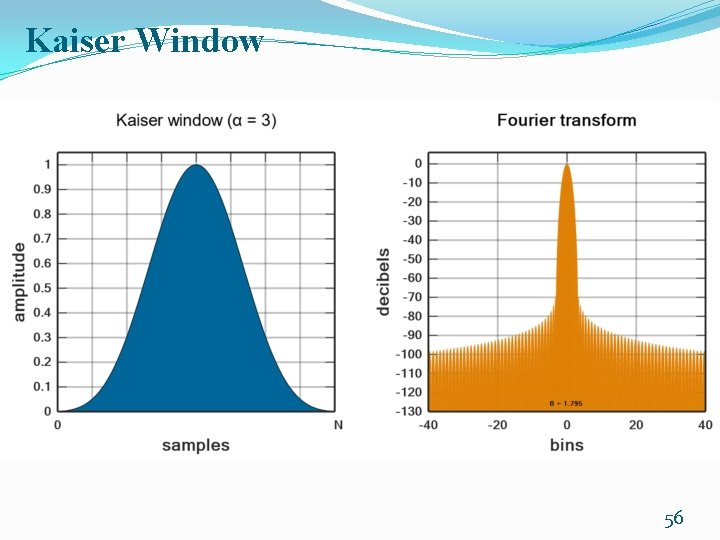
Kaiser Window �A trade-off between the size of the sidelobe and the width of the mainlobe can be achieved by changing the length of the window and the parameter a. 55

Kaiser Window 56

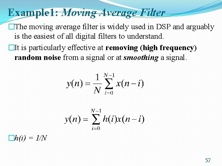
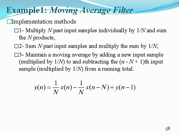
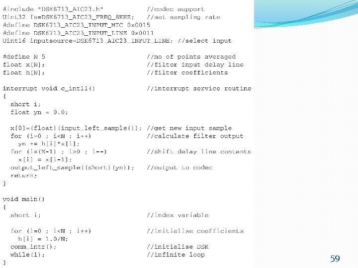
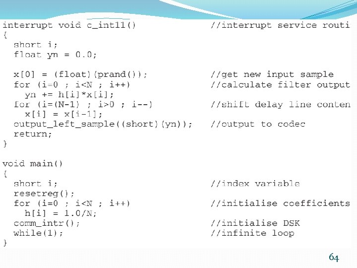
Example 1: Moving Average Filter �The moving average filter is widely used in DSP and arguably is the easiest of all digital filters to understand. �It is particularly effective at removing (high frequency) random noise from a signal or at smoothing a signal. �h(i) = 1/N 57

Example 1: Moving Average Filter �Implementation methods � 1 - Multiply N past input samples individually by 1/N and sum the N products, � 2 - Sum N past input samples and multiply the sum by 1/N, � 3 - Maintain a moving average by adding a new input sample (multiplied by 1/N) to and subtracting the (n - N + 1)th input sample (multiplied by 1/N) from a running total. 58

59

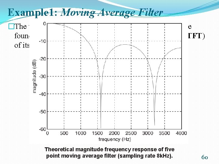
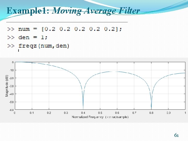
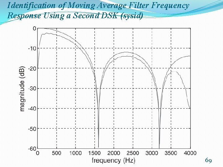
Example 1: Moving Average Filter �The theoretical frequency response of the filter can be found by taking the discrete time Fourier transform (DTFT) of its coefficients: Theoretical magnitude frequency response of five point moving average filter (sampling rate 8 k. Hz). 60

Example 1: Moving Average Filter 61

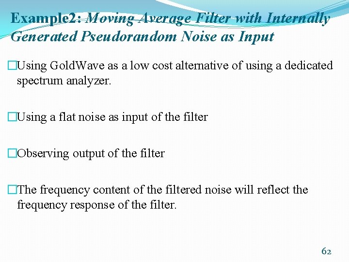
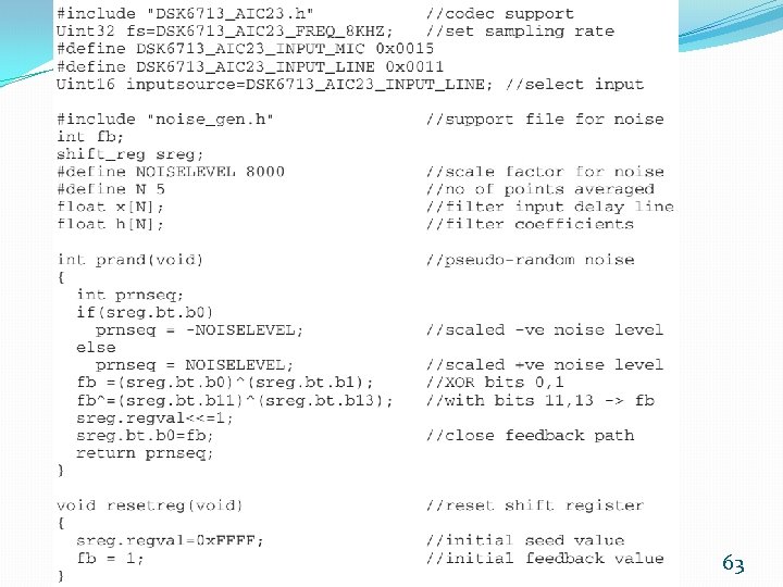
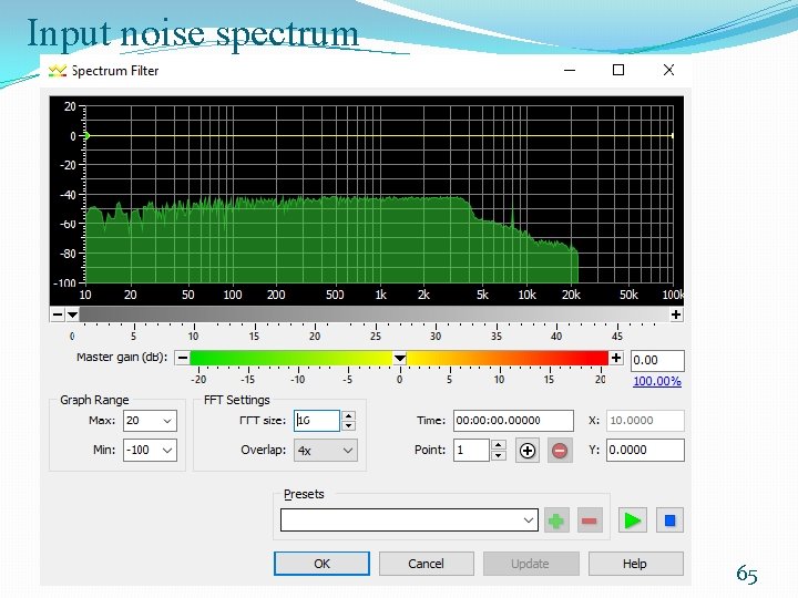
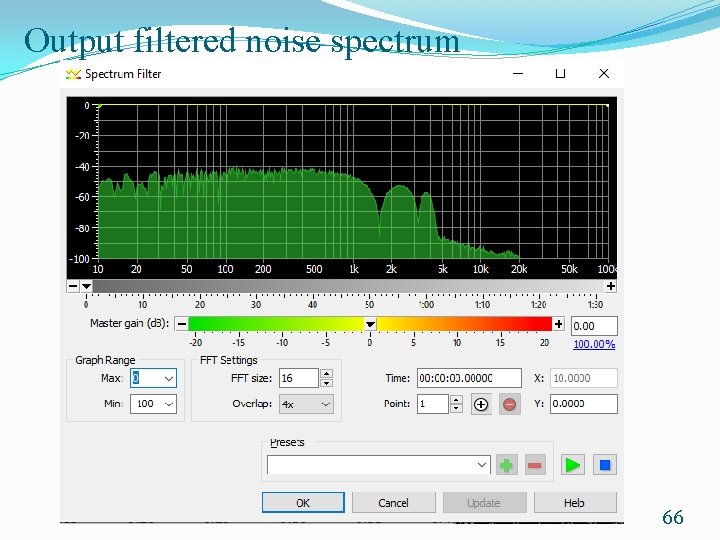
Example 2: Moving Average Filter with Internally Generated Pseudorandom Noise as Input �Using Gold. Wave as a low cost alternative of using a dedicated spectrum analyzer. �Using a flat noise as input of the filter �Observing output of the filter �The frequency content of the filtered noise will reflect the frequency response of the filter. 62

63

64

Input noise spectrum 65

Output filtered noise spectrum 66

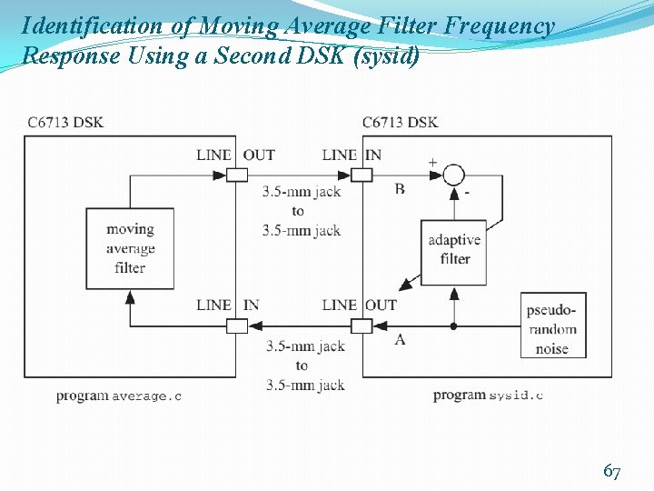
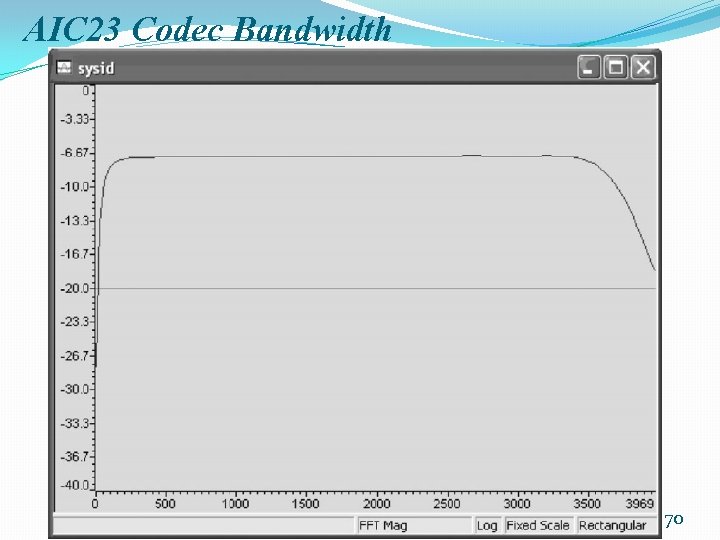
Identification of Moving Average Filter Frequency Response Using a Second DSK (sysid) 67

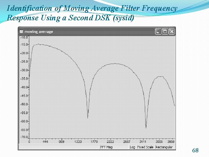
Identification of Moving Average Filter Frequency Response Using a Second DSK (sysid) 68

Identification of Moving Average Filter Frequency Response Using a Second DSK (sysid) 69

AIC 23 Codec Bandwidth 70

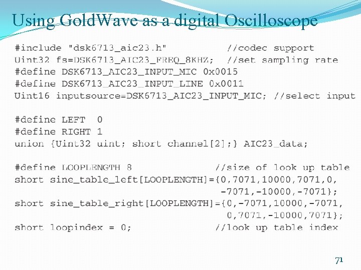
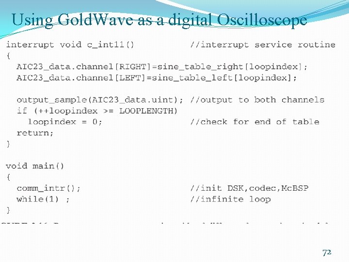
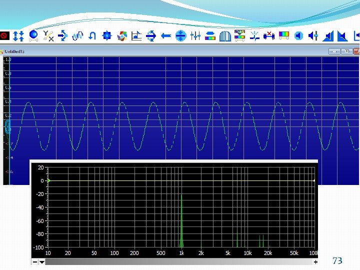
Using Gold. Wave as a digital Oscilloscope 71

Using Gold. Wave as a digital Oscilloscope 72

73

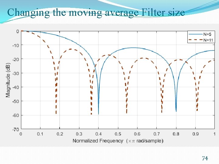
Changing the moving average Filter size 74

Windowing function 75

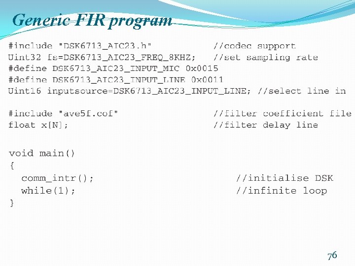
Generic FIR program 76

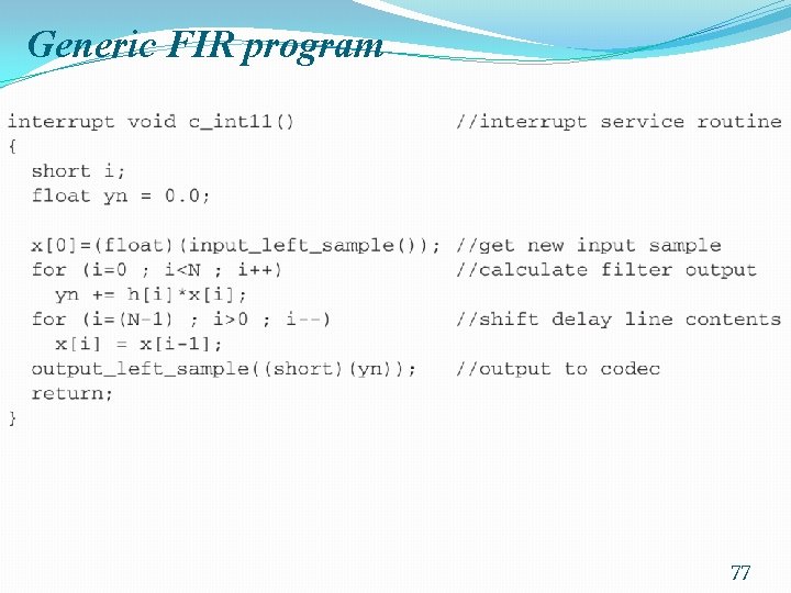
Generic FIR program 77

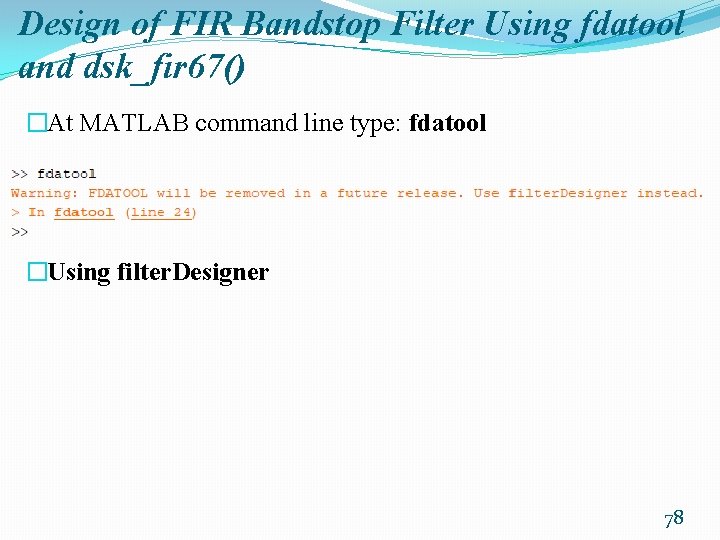
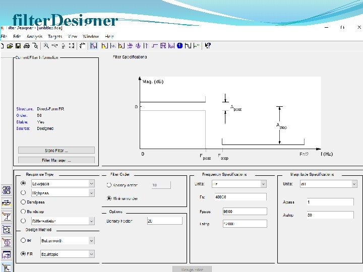
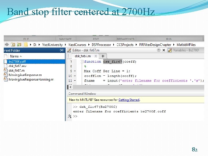
Design of FIR Bandstop Filter Using fdatool and dsk_fir 67() �At MATLAB command line type: fdatool �Using filter. Designer 78

filter. Designer 79

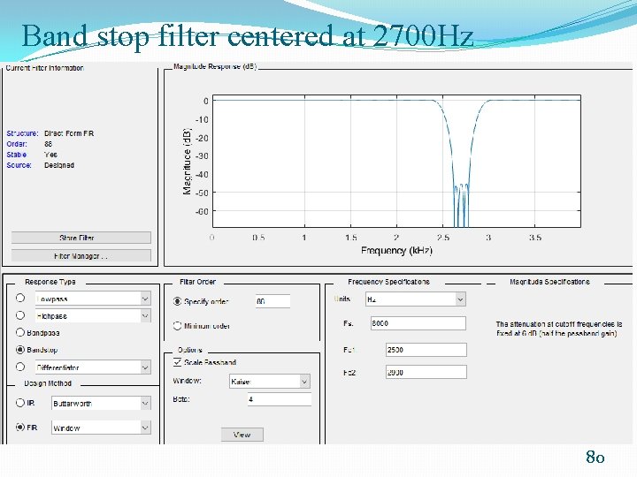
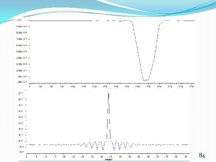
Band stop filter centered at 2700 Hz 80

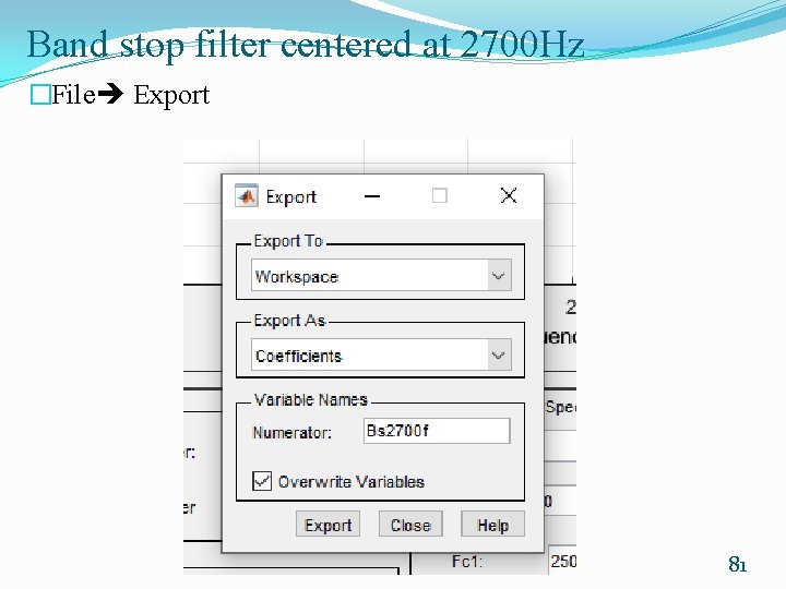
Band stop filter centered at 2700 Hz �File Export 81

Band stop filter centered at 2700 Hz 82

MATLAB M-file 83

84

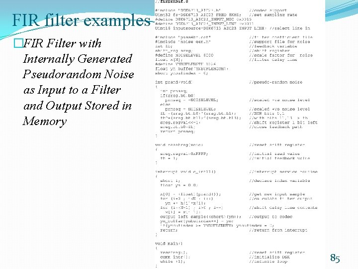
FIR filter examples �FIR Filter with Internally Generated Pseudorandom Noise as Input to a Filter and Output Stored in Memory 85

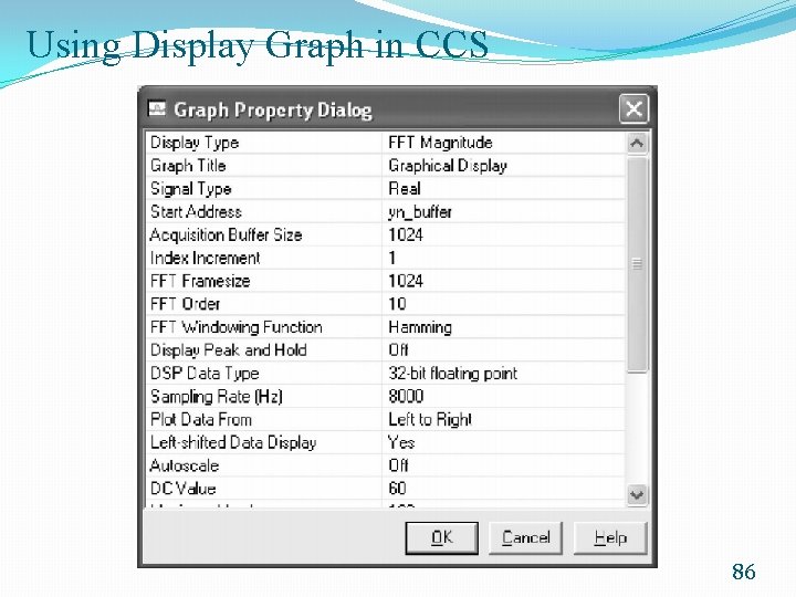
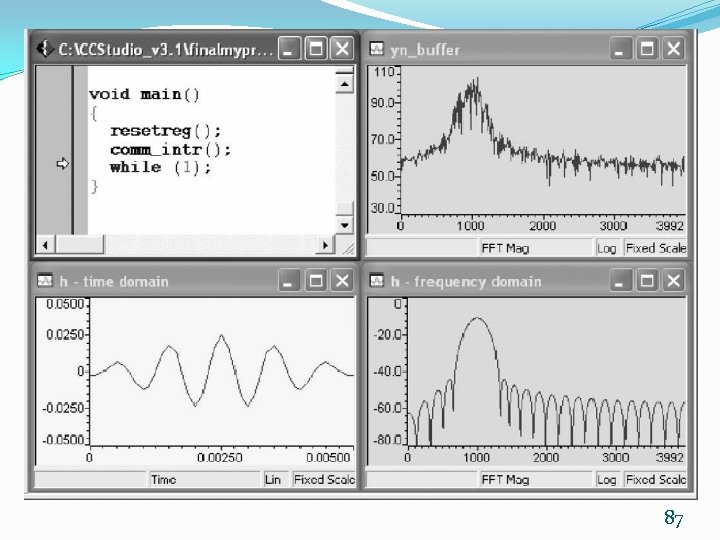
Using Display Graph in CCS 86

87

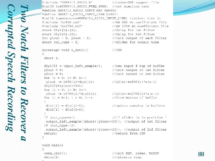
Two Notch Filters to Recover a Corrupted Speech Recording 88

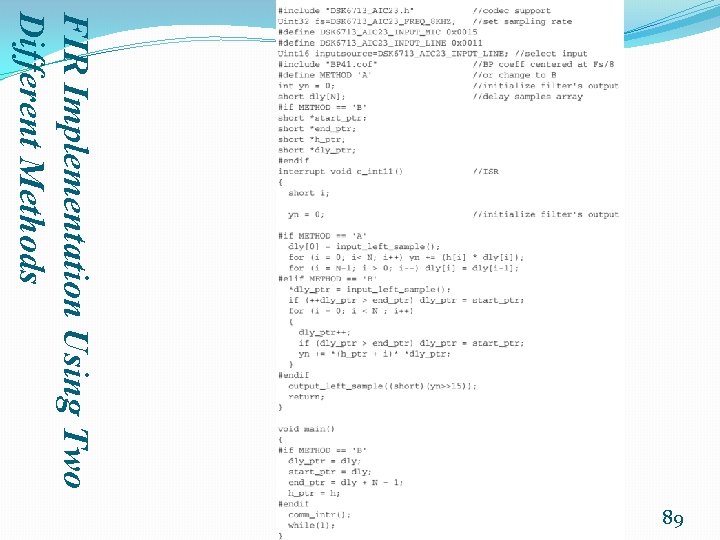
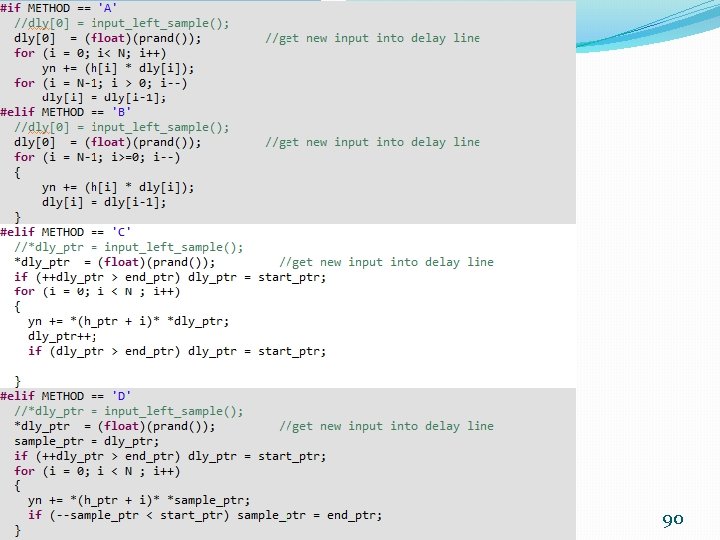
FIR Implementation Using Two Different Methods 89

90

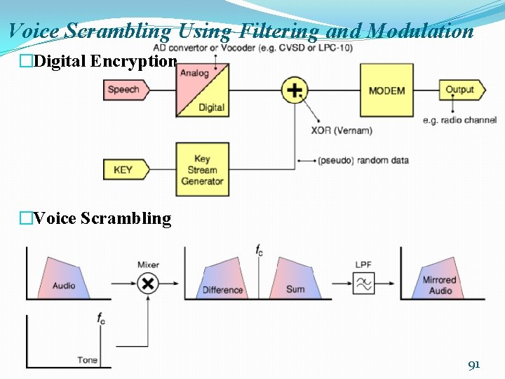
Voice Scrambling Using Filtering and Modulation �Digital Encryption �Voice Scrambling 91