1 CSCI 104 Graph Algorithms Mark Redekopp 2

1 CSCI 104 Graph Algorithms Mark Redekopp

2 PAGERANK ALGORITHM

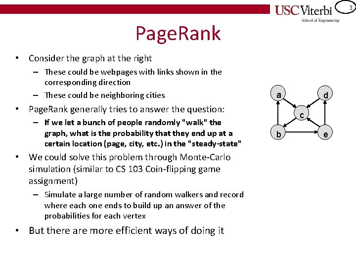
3 Page. Rank • Consider the graph at the right – These could be webpages with links shown in the corresponding direction – These could be neighboring cities a • Page. Rank generally tries to answer the question: – If we let a bunch of people randomly "walk" the graph, what is the probability that they end up at a certain location (page, city, etc. ) in the "steady-state" • We could solve this problem through Monte-Carlo simulation (similar to CS 103 Coin-flipping game assignment) – Simulate a large number of random walkers and record where each one ends to build up an answer of the probabilities for each vertex • But there are more efficient ways of doing it d c b e

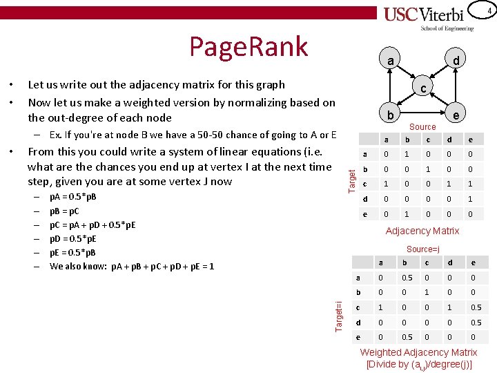
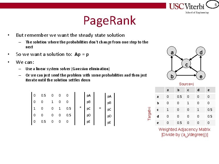
4 Page. Rank • • a Let us write out the adjacency matrix for this graph Now let us make a weighted version by normalizing based on the out-degree of each node c b p. A = 0. 5*p. B = p. C = p. A + p. D + 0. 5*p. E p. D = 0. 5*p. E = 0. 5*p. B We also know: p. A + p. B + p. C + p. D + p. E = 1 a d e a 0 1 0 0 0 b 0 0 1 0 0 c 1 0 0 1 1 d 0 0 1 e 0 1 0 0 0 Adjacency Matrix Source=j Target=i – – – Target From this you could write a system of linear equations (i. e. what are the chances you end up at vertex I at the next time step, given you are at some vertex J now e Source b c – Ex. If you're at node B we have a 50 -50 chance of going to A or E • d a b c d e a 0 0. 5 0 0 0 b 0 0 1 0 0 c 1 0 0 1 0. 5 d 0 0 0. 5 e 0 0. 5 0 0 0 Weighted Adjacency Matrix [Divide by (ai, j)/degree(j)]

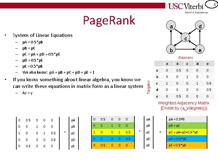
5 Page. Rank c p. A = 0. 5*p. B = p. C = p. A + p. D + 0. 5*p. E p. D = 0. 5*p. E = 0. 5*p. B We also know: p. A + p. B + p. C + p. D + p. E = 1 – – – • d System of Linear Equations b e Source=j If you know something about linear algebra, you know we can write these equations in matrix form as a linear system – Ax = y Target=i • a a b c d e a 0 0. 5 0 0 0 b 0 0 1 0 0 c 1 0 0 1 0. 5 d 0 0 0. 5 e 0 0. 5 0 0 0 Weighted Adjacency Matrix [Divide by (ai, j)/degree(j)] 0 0. 5 0 0 0 p. A = 0. 5 PB 0 0 1 0 0 p. B = p. C 1 0 0 1 0. 5 0 0 0 0 0. 5 p. D = 0. 5*p. E 0 0. 5 0 0 0 p. E = 0. 5*p. B * * p. C = p. A+p. D+0. 5*p. E

6 Page. Rank • But remember we want the steady state solution – The solution where the probabilities don't change from one step to the next a So we want a solution to: Ap = p We can: d c – Use a linear system solver (Gaussian elimination) – Or we can just seed the problem with some probabilities and then just iterate until the solution settles down b e Source=j a b c d e 0 0. 5 0 0 0 p. A a 0 0. 5 0 0 0 1 0 0 p. B b 0 0 1 0. 5 c 1 0 0 1 0. 5 0 0 0. 5 p. D d 0 0 0. 5 0 0 0 p. E e 0 0. 5 0 0 0 * p. C = p. C Target=i • • Weighted Adjacency Matrix [Divide by (ai, j)/degree(j)]

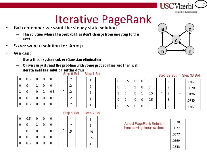
7 • Iterative Page. Rank But remember we want the steady state solution – The solution where the probabilities don't change from one step to the next • • a d c So we want a solution to: Ap = p We can: b e – Use a linear system solver (Gaussian elimination) – Or we can just seed the problem with some probabilities and then just iterate until the solution settles down Step 0 Sol. Step 1 Sol. Step 29 Sol. Step 30 Sol. 0 0. 5 0 0 0 . 2 . 1 0 0. 5 0 0 0 ? 0 0 1 0 0 . 2 . 1507 . 2 0 0 1 0 0 ? 1 0 0 1 0. 5 . 3078 . 5 1 0 0 1 0. 5 0 0 0. 5 . 2 . 1 0 0 0. 5 ? 0 0. 5 0 0 0 . 2 . 0783 . 1 0 0. 5 0 0 0 ? . 1507 * . 2 = Step 1 Sol. 0. 5 0 0 0 . 1 0 0 . 2 . 5 1 0 0 1 0. 5 0 0 0. 5 . 1 . 05 0 0 0 . 1 . 5 ? = Step 2 Sol. 0 * * = . 25 Actual Page. Rank Solution from solving linear system: . 1538. 3077. 0769. 1538 . 3126

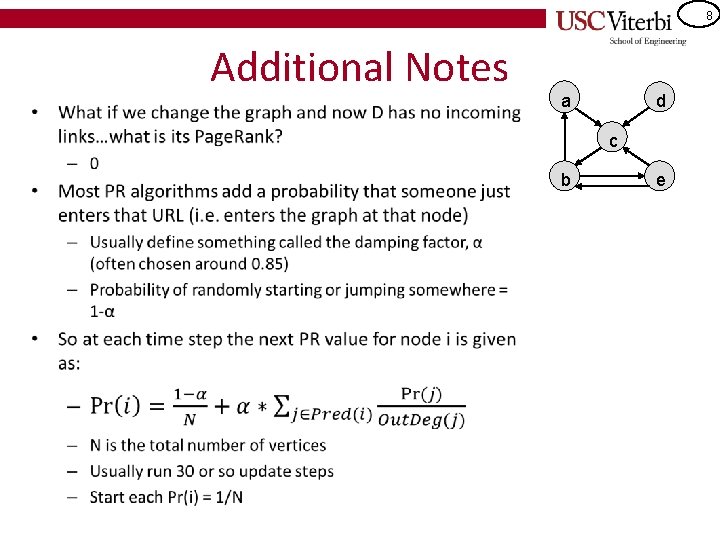
8 Additional Notes • a d c b e

9 In a Web Search Setting • • Given some search keywords we could find the pages that have that matching keywords We often expand that set of pages by including all successors and predecessors of those pages – Include all pages that are within a radius of 1 of the pages that actually have the keyword • • Now consider that set of pages and the subgraph that it induces Run Page. Rank on that subgraph Full Web. Graph Page Hits (Contain keyword) Expanded (Preds & Succs) g g g a d a c b a c e f d b d a c e f Induced Subgraph to run Page. Rank b c e f d b e

10 Dijkstra's Algorithm SINGLE-SOURCE SHORTEST PATH (SSSP)

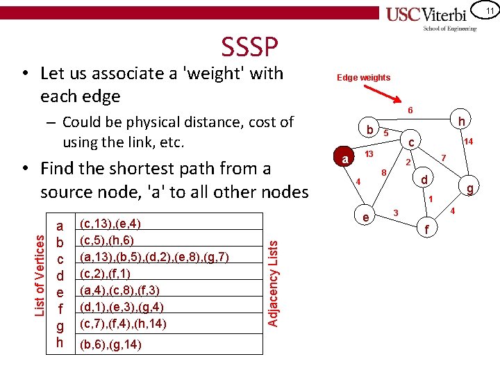
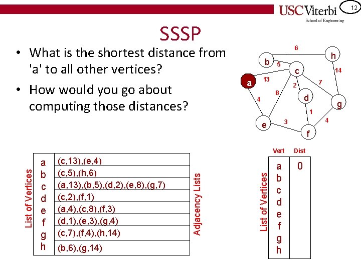
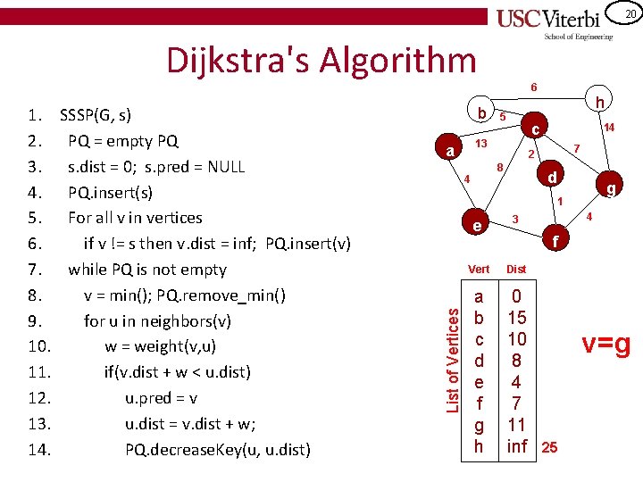
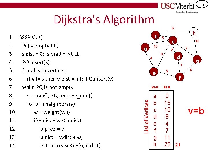
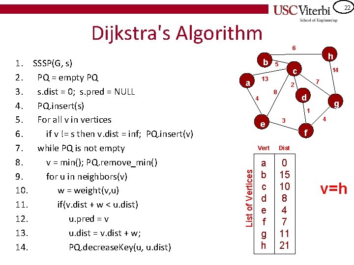
11 SSSP • Let us associate a 'weight' with each edge Edge weights 6 – Could be physical distance, cost of using the link, etc. a b c d e f g h (c, 13), (e, 4) (c, 5), (h, 6) (a, 13), (b, 5), (d, 2), (e, 8), (g, 7) (c, 2), (f, 1) (a, 4), (c, 8), (f, 3) (d, 1), (e, 3), (g, 4) (c, 7), (f, 4), (h, 14) (b, 6), (g, 14) 5 14 7 2 8 4 h c 13 a d g 1 e Adjacency Lists List of Vertices • Find the shortest path from a source node, 'a' to all other nodes b 4 3 f

12 SSSP • What is the shortest distance from 'a' to all other vertices? • How would you go about computing those distances? 6 b 5 (b, 6), (g, 14) d g 1 List of Vertices Adjacency Lists List of Vertices (c, 13), (e, 4) (c, 5), (h, 6) (a, 13), (b, 5), (d, 2), (e, 8), (g, 7) (c, 2), (f, 1) (a, 4), (c, 8), (f, 3) (d, 1), (e, 3), (g, 4) (c, 7), (f, 4), (h, 14) 7 8 4 14 2 4 3 e a b c d e f g h c 13 a h f Vert Dist a b c d e f g h 0

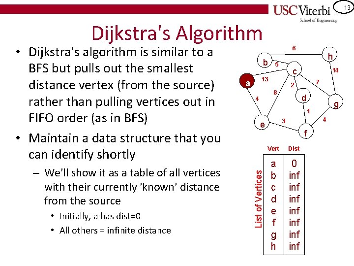
13 Dijkstra's Algorithm – We'll show it as a table of all vertices with their currently 'known' distance from the source • Initially, a has dist=0 • All others = infinite distance 6 b 5 14 7 2 8 4 h c 13 a d g 1 4 3 e List of Vertices • Dijkstra's algorithm is similar to a BFS but pulls out the smallest distance vertex (from the source) rather than pulling vertices out in FIFO order (as in BFS) • Maintain a data structure that you can identify shortly f Vert Dist a b c d e f g h 0 inf inf

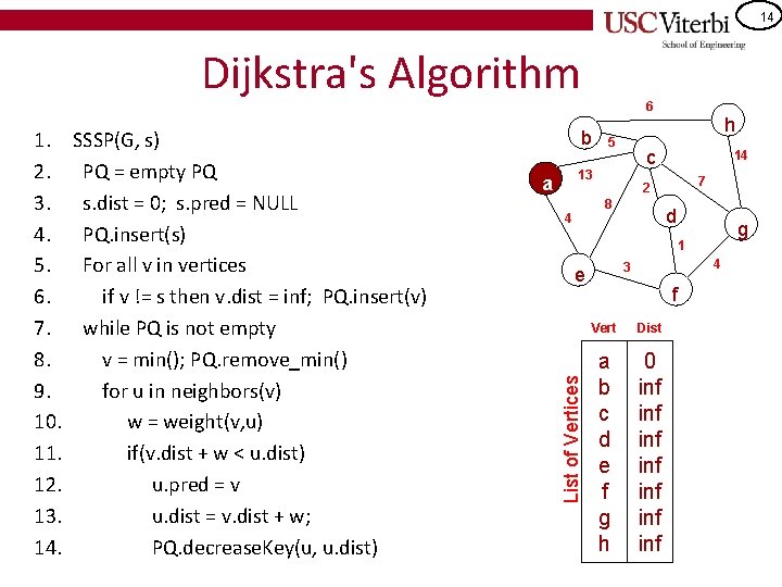
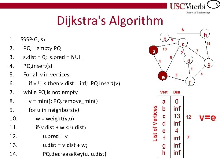
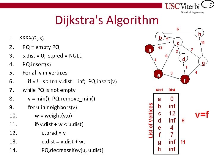
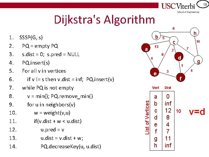
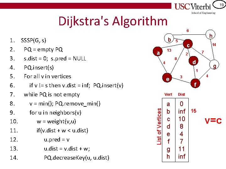
14 Dijkstra's Algorithm SSSP(G, s) PQ = empty PQ s. dist = 0; s. pred = NULL PQ. insert(s) For all v in vertices if v != s then v. dist = inf; PQ. insert(v) while PQ is not empty v = min(); PQ. remove_min() for u in neighbors(v) w = weight(v, u) if(v. dist + w < u. dist) u. pred = v u. dist = v. dist + w; PQ. decrease. Key(u, u. dist) b 5 14 7 2 8 4 h c 13 a d g 1 4 3 e List of Vertices 1. 2. 3. 4. 5. 6. 7. 8. 9. 10. 11. 12. 13. 14. 6 f Vert Dist a b c d e f g h 0 inf inf

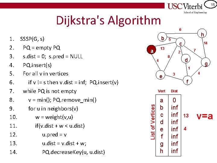
15 Dijkstra's Algorithm SSSP(G, s) PQ = empty PQ s. dist = 0; s. pred = NULL PQ. insert(s) For all v in vertices if v != s then v. dist = inf; PQ. insert(v) while PQ is not empty v = min(); PQ. remove_min() for u in neighbors(v) w = weight(v, u) if(v. dist + w < u. dist) u. pred = v u. dist = v. dist + w; PQ. decrease. Key(u, u. dist) b 5 14 7 2 8 4 h c 13 a d g 1 List of Vertices 1. 2. 3. 4. 5. 6. 7. 8. 9. 10. 11. 12. 13. 14. 6 e 3 Vert Dist a b c d e f g h 0 inf inf 4 f 13 4 v=a

16 Dijkstra's Algorithm SSSP(G, s) PQ = empty PQ s. dist = 0; s. pred = NULL PQ. insert(s) For all v in vertices if v != s then v. dist = inf; PQ. insert(v) while PQ is not empty v = min(); PQ. remove_min() for u in neighbors(v) w = weight(v, u) if(v. dist + w < u. dist) u. pred = v u. dist = v. dist + w; PQ. decrease. Key(u, u. dist) b 5 14 7 2 8 4 h c 13 a d g 1 List of Vertices 1. 2. 3. 4. 5. 6. 7. 8. 9. 10. 11. 12. 13. 14. 6 e 3 Vert Dist a b c d e f g h 0 inf 13 inf 4 inf inf 4 f 12 7 v=e

17 Dijkstra's Algorithm SSSP(G, s) PQ = empty PQ s. dist = 0; s. pred = NULL PQ. insert(s) For all v in vertices if v != s then v. dist = inf; PQ. insert(v) while PQ is not empty v = min(); PQ. remove_min() for u in neighbors(v) w = weight(v, u) if(v. dist + w < u. dist) u. pred = v u. dist = v. dist + w; PQ. decrease. Key(u, u. dist) b 5 14 7 2 8 4 h c 13 a d g 1 List of Vertices 1. 2. 3. 4. 5. 6. 7. 8. 9. 10. 11. 12. 13. 14. 6 e 3 Vert Dist a b c d e f g h 0 inf 12 inf 4 7 inf 4 f 8 11 v=f

18 Dijkstra's Algorithm SSSP(G, s) PQ = empty PQ s. dist = 0; s. pred = NULL PQ. insert(s) For all v in vertices if v != s then v. dist = inf; PQ. insert(v) while PQ is not empty v = min(); PQ. remove_min() for u in neighbors(v) w = weight(v, u) if(v. dist + w < u. dist) u. pred = v u. dist = v. dist + w; PQ. decrease. Key(u, u. dist) b 5 14 7 2 8 4 h c 13 a d g 1 List of Vertices 1. 2. 3. 4. 5. 6. 7. 8. 9. 10. 11. 12. 13. 14. 6 e 3 Vert Dist a b c d e f g h 0 inf 12 8 4 7 11 inf 4 f 10 v=d

19 Dijkstra's Algorithm SSSP(G, s) PQ = empty PQ s. dist = 0; s. pred = NULL PQ. insert(s) For all v in vertices if v != s then v. dist = inf; PQ. insert(v) while PQ is not empty v = min(); PQ. remove_min() for u in neighbors(v) w = weight(v, u) if(v. dist + w < u. dist) u. pred = v u. dist = v. dist + w; PQ. decrease. Key(u, u. dist) b 5 14 7 2 8 4 h c 13 a d g 1 List of Vertices 1. 2. 3. 4. 5. 6. 7. 8. 9. 10. 11. 12. 13. 14. 6 e 3 Vert Dist a b c d e f g h 0 inf 10 8 4 7 11 inf 4 f 15 v=c

20 Dijkstra's Algorithm SSSP(G, s) PQ = empty PQ s. dist = 0; s. pred = NULL PQ. insert(s) For all v in vertices if v != s then v. dist = inf; PQ. insert(v) while PQ is not empty v = min(); PQ. remove_min() for u in neighbors(v) w = weight(v, u) if(v. dist + w < u. dist) u. pred = v u. dist = v. dist + w; PQ. decrease. Key(u, u. dist) b 5 14 7 2 8 4 h c 13 a d g 1 List of Vertices 1. 2. 3. 4. 5. 6. 7. 8. 9. 10. 11. 12. 13. 14. 6 e 3 Vert Dist a b c d e f g h 0 15 10 8 4 7 11 inf 4 f v=g 25

21 Dijkstra's Algorithm SSSP(G, s) PQ = empty PQ s. dist = 0; s. pred = NULL PQ. insert(s) For all v in vertices if v != s then v. dist = inf; PQ. insert(v) while PQ is not empty v = min(); PQ. remove_min() for u in neighbors(v) w = weight(v, u) if(v. dist + w < u. dist) u. pred = v u. dist = v. dist + w; PQ. decrease. Key(u, u. dist) b 5 14 7 2 8 4 h c 13 a d g 1 List of Vertices 1. 2. 3. 4. 5. 6. 7. 8. 9. 10. 11. 12. 13. 14. 6 e 3 Vert Dist a b c d e f g h 0 15 10 8 4 7 11 25 4 f v=b 21

22 Dijkstra's Algorithm SSSP(G, s) PQ = empty PQ s. dist = 0; s. pred = NULL PQ. insert(s) For all v in vertices if v != s then v. dist = inf; PQ. insert(v) while PQ is not empty v = min(); PQ. remove_min() for u in neighbors(v) w = weight(v, u) if(v. dist + w < u. dist) u. pred = v u. dist = v. dist + w; PQ. decrease. Key(u, u. dist) b 5 14 7 2 8 4 h c 13 a d g 1 List of Vertices 1. 2. 3. 4. 5. 6. 7. 8. 9. 10. 11. 12. 13. 14. 6 e 3 Vert Dist a b c d e f g h 0 15 10 8 4 7 11 21 4 f v=h

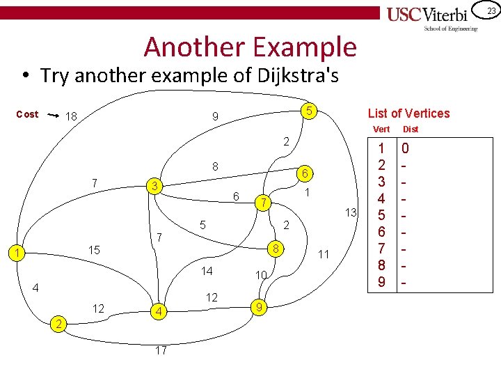
23 Another Example • Try another example of Dijkstra's Cost 18 5 9 List of Vertices Vert 2 8 7 3 6 6 1 7 5 2 7 8 15 1 14 4 12 12 4 2 17 13 10 9 11 1 2 3 4 5 6 7 8 9 Dist 0 -

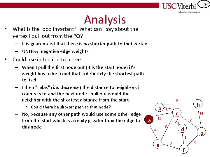
24 Analysis • What is the loop invariant? What can I say about the vertex I pull out from the PQ? – It is guaranteed that there is no shorter path to that vertex – UNLESS: negative edge weights • Could use induction to prove – When I pull the first node out (it is the start node) it's weight has to be 0 and that is definitely the shortest path to itself – I then "relax" (i. e. decrease) the distance to neighbors it connects to and the next node I pull out would the neighbor with the shortest distance from the start 6 • Could there be shorter path to that node? – No, because any other path would use some other edge from the start which is already greater than the edge to this node b 5 c 13 a 14 7 2 8 4 h d g 1 e 4 3 f

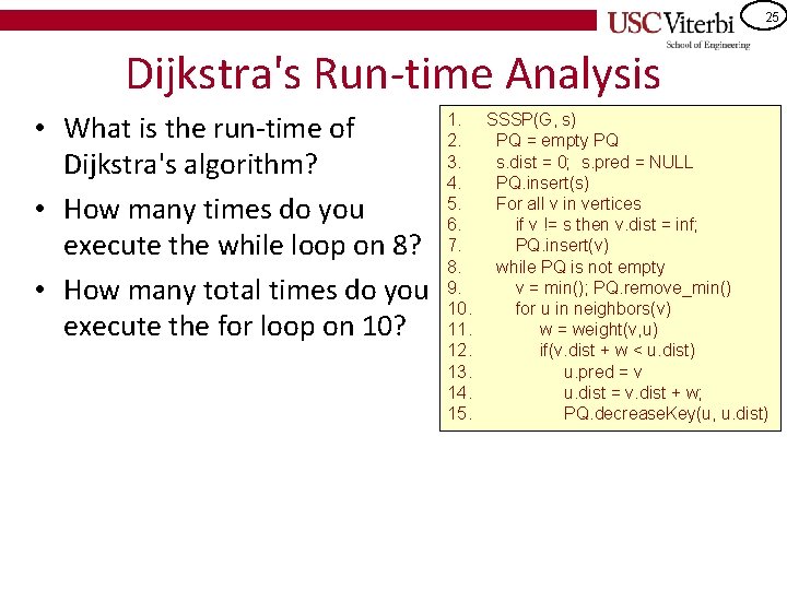
25 Dijkstra's Run-time Analysis • What is the run-time of Dijkstra's algorithm? • How many times do you execute the while loop on 8? • How many total times do you execute the for loop on 10? 1. SSSP(G, s) 2. PQ = empty PQ 3. s. dist = 0; s. pred = NULL 4. PQ. insert(s) 5. For all v in vertices 6. if v != s then v. dist = inf; 7. PQ. insert(v) 8. while PQ is not empty 9. v = min(); PQ. remove_min() 10. for u in neighbors(v) 11. w = weight(v, u) 12. if(v. dist + w < u. dist) 13. u. pred = v 14. u. dist = v. dist + w; 15. PQ. decrease. Key(u, u. dist)

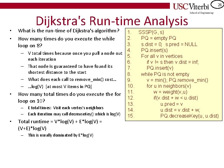
26 • • Dijkstra's Run-time Analysis What is the run-time of Dijkstra's algorithm? How many times do you execute the while loop on 8? 1. SSSP(G, s) 2. PQ = empty PQ 3. s. dist = 0; s. pred = NULL 4. PQ. insert(s) – V total times because once you pull a node out 5. For all v in vertices each iteration 6. if v != s then v. dist = inf; – That node is guaranteed to have found its 7. PQ. insert(v) shortest distance to the start 8. while PQ is not empty – What does each call to remove_min() cost… 9. v = min(); PQ. remove_min() 10. for u in neighbors(v) – …log(V) [at most V items in PQ] w = weight(v, u) How many total times do you execute the for 11. 12. if(v. dist + w < u. dist) loop on 10? 13. u. pred = v – E total times: Visit each vertex's neighbors 14. u. dist = v. dist + w; – Each iteration may call decrease. Key() which is log(V) 15. PQ. decrease. Key(u, u. dist) Total runtime = V*log(V) + E*log(V) = (V+E)*log(V) – This is usually dominated by E*log(V)

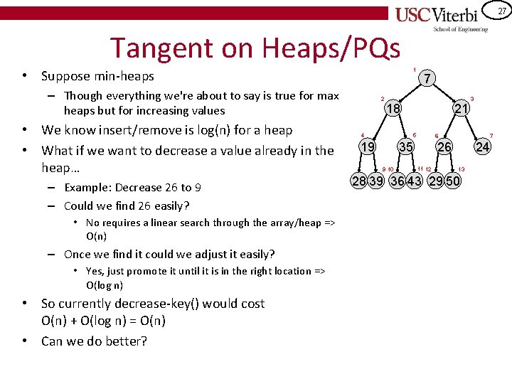
27 Tangent on Heaps/PQs 1 • Suppose min-heaps – Though everything we're about to say is true for max heaps but for increasing values • We know insert/remove is log(n) for a heap • What if we want to decrease a value already in the heap… – Example: Decrease 26 to 9 – Could we find 26 easily? • No requires a linear search through the array/heap => O(n) – Once we find it could we adjust it easily? • Yes, just promote it until it is in the right location => O(log n) • So currently decrease-key() would cost O(n) + O(log n) = O(n) • Can we do better? 2 7 18 4 21 5 19 6 35 9 10 3 7 26 11 12 24 13 28 39 36 43 29 50

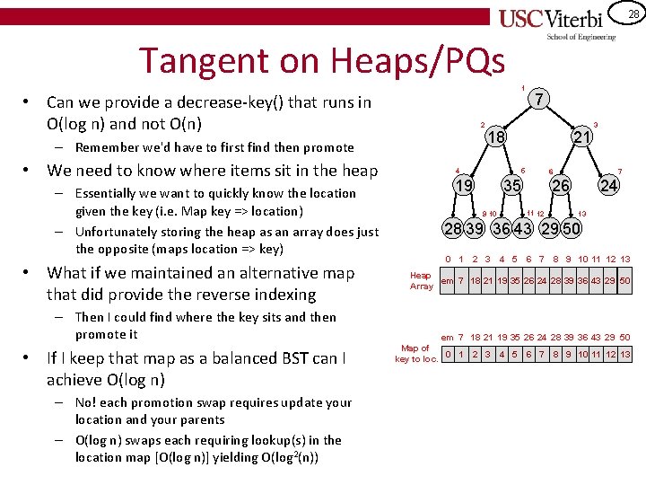
28 Tangent on Heaps/PQs 1 • Can we provide a decrease-key() that runs in O(log n) and not O(n) 2 – Remember we'd have to first find then promote • We need to know where items sit in the heap – Essentially we want to quickly know the location given the key (i. e. Map key => location) – Unfortunately storing the heap as an array does just the opposite (maps location => key) • What if we maintained an alternative map that did provide the reverse indexing – Then I could find where the key sits and then promote it • If I keep that map as a balanced BST can I achieve O(log n) – No! each promotion swap requires update your location and your parents – O(log n) swaps each requiring lookup(s) in the location map [O(log n)] yielding O(log 2(n)) 7 18 4 21 5 19 6 35 7 26 11 12 9 10 3 24 13 28 39 36 43 29 50 0 1 2 3 4 5 6 7 8 9 10 11 12 13 Heap em 7 18 21 19 35 26 24 28 39 36 43 29 50 Array em 7 18 21 19 35 26 24 28 39 36 43 29 50 Map of key to loc. 0 1 2 3 4 5 6 7 8 9 10 11 12 13

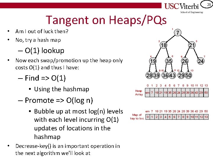
29 Tangent on Heaps/PQs • Am I out of luck then? • No, try a hash map – O(1) lookup • Now each swap/promotion up the heap only costs O(1) and thus I have: – Find => O(1) • Using the hashmap – Promote => O(log n) • Bubble up at most log(n) levels with each level incurring O(1) updates of locations in the hashmap • Decrease-key() is an important operation in the next algorithm we'll look at 1 2 7 18 4 21 5 19 6 35 7 26 11 12 9 10 3 24 13 28 39 36 43 29 50 0 1 2 3 4 5 6 7 8 9 10 11 12 13 Heap em 7 18 21 19 35 26 24 28 39 36 43 29 50 Array em 7 18 21 19 35 26 24 28 39 36 43 29 50 Map of key to loc. 0 1 2 3 4 5 6 7 8 9 10 11 12 13

30 A* Search Algorithm ALGORITHM HIGHLIGHT

31 Search Methods • Many systems require searching for goal states – Path Planning • Roomba Vacuum • Mapquest/Google Maps • Games!! – Optimization Problems • Find the optimal solution to a problem with many constraints

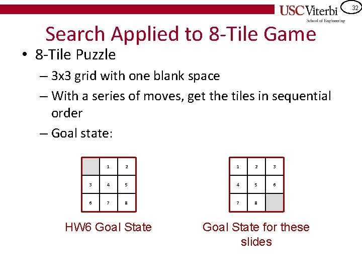
32 Search Applied to 8 -Tile Game • 8 -Tile Puzzle – 3 x 3 grid with one blank space – With a series of moves, get the tiles in sequential order – Goal state: 1 2 3 3 4 5 6 6 7 8 HW 6 Goal State for these slides

33 Search Methods • Brute-Force Search: When you don’t know where the answer is, just search all possibilities until you find it. • Heuristic Search: A heuristic is a “rule of thumb”. An example is in a chess game, to decide which move to make, count the values of the pieces left for your opponent. Use that value to “score” the possible moves you can make. – Heuristics are not perfect measures, they are quick computations to give an approximation (e. g. may not take into account “delayed gratification” or “setting up an opponent”)

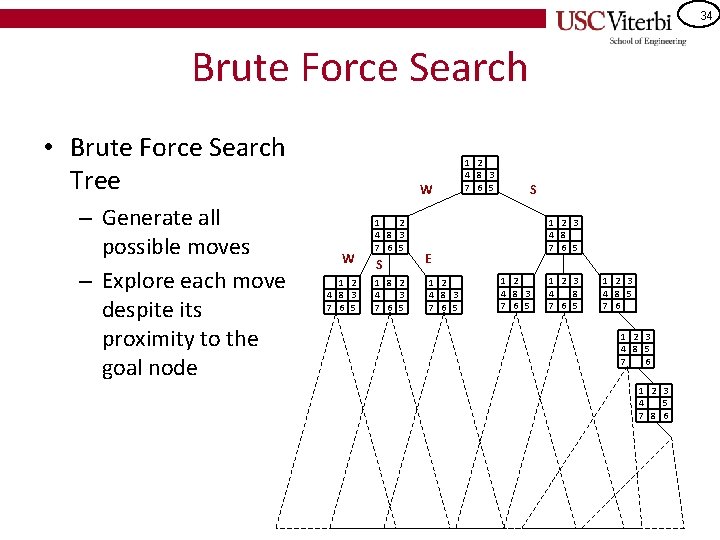
34 Brute Force Search • Brute Force Search Tree – Generate all possible moves – Explore each move despite its proximity to the goal node W W 1 2 4 8 3 7 6 5 S 1 8 2 4 3 7 6 5 1 2 4 8 3 7 6 5 S 1 2 3 4 8 7 6 5 E 1 2 4 8 3 7 6 5 1 2 3 4 8 5 7 6 1 2 3 4 5 7 8 6

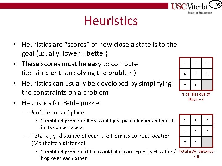
35 Heuristics • Heuristics are “scores” of how close a state is to the goal (usually, lower = better) • These scores must be easy to compute (i. e. simpler than solving the problem) • Heuristics can usually be developed by simplifying the constraints on a problem • Heuristics for 8 -tile puzzle 1 8 3 4 5 6 2 7 # of Tiles out of Place = 3 – # of tiles out of place • Simplified problem: If we could just pick a tile up and put it in its correct place – Total x-, y- distance of each tile from its correct location (Manhattan distance) 1 8 3 4 5 6 2 7 • Simplified problem if tiles could stack on top of each other / Total x-/y- distance =6 hop over each other

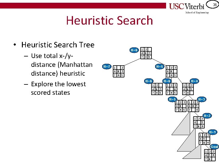
36 Heuristic Search • Heuristic Search Tree – Use total x-/y- distance (Manhattan distance) heuristic – Explore the lowest scored states H=6 H=7 1 2 4 8 3 7 6 5 H=5 1 2 4 8 3 7 6 5 H=6 1 2 3 4 8 7 6 5 H=5 H=4 1 2 3 4 8 5 7 6 1 2 3 4 8 7 6 5 1 2 3 4 8 5 7 6 H=3 1 2 3 4 5 7 8 6 H=2 1 2 3 4 5 7 8 6 H=1 Goal 1 2 3 4 5 6 7 8

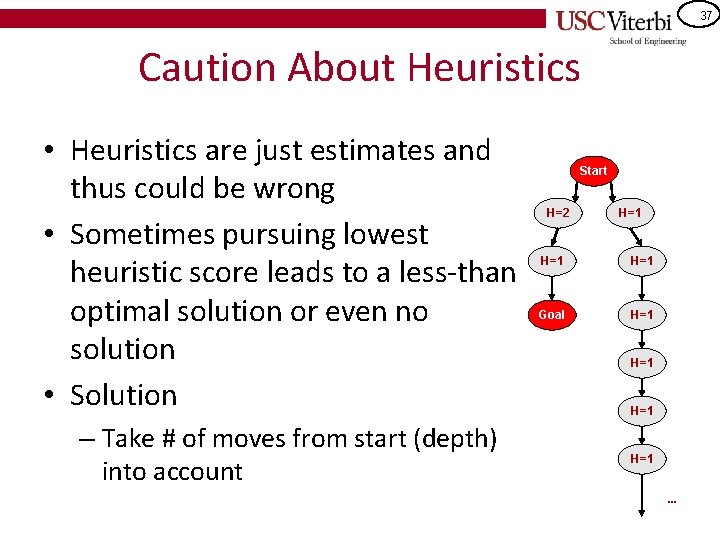
37 Caution About Heuristics • Heuristics are just estimates and thus could be wrong • Sometimes pursuing lowest heuristic score leads to a less-than optimal solution or even no solution • Solution – Take # of moves from start (depth) into account Start H=2 H=1 H=1 Goal H=1 H=1 …

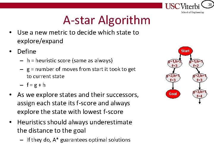
38 A-star Algorithm • Use a new metric to decide which state to explore/expand • Define – h = heuristic score (same as always) – g = number of moves from start it took to get to current state – f = g + h • As we explore states and their successors, assign each state its f-score and always explore the state with lowest f-score • Heuristics should always underestimate the distance to the goal – If they do, A* guarantees optimal solutions Start g=1, h=2 f=3 g=1, h=1 f=2 g=2, h=1 f=3 Goal g=3, h=1 f=4

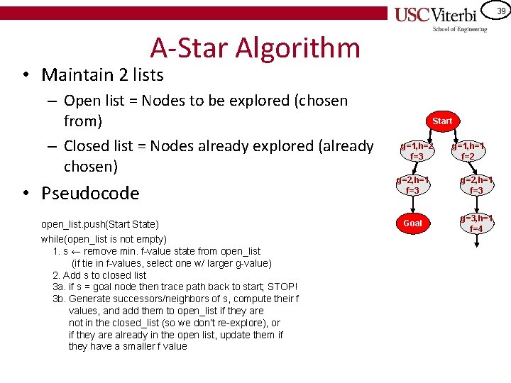
39 A-Star Algorithm • Maintain 2 lists – Open list = Nodes to be explored (chosen from) – Closed list = Nodes already explored (already chosen) • Pseudocode open_list. push(Start State) while(open_list is not empty) 1. s ← remove min. f-value state from open_list (if tie in f-values, select one w/ larger g-value) 2. Add s to closed list 3 a. if s = goal node then trace path back to start; STOP! 3 b. Generate successors/neighbors of s, compute their f values, and add them to open_list if they are not in the closed_list (so we don’t re-explore), or if they are already in the open list, update them if they have a smaller f value Start g=1, h=2 f=3 g=1, h=1 f=2 g=2, h=1 f=3 Goal g=3, h=1 f=4

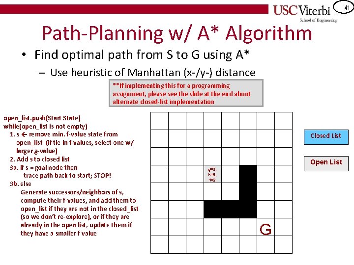
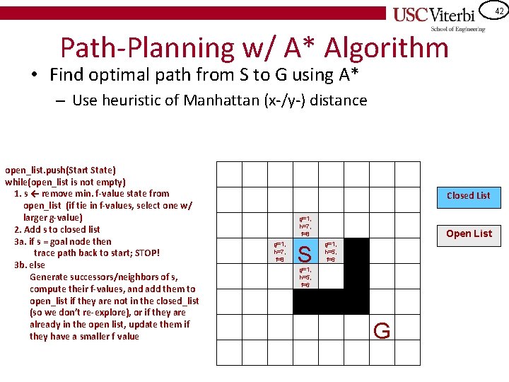
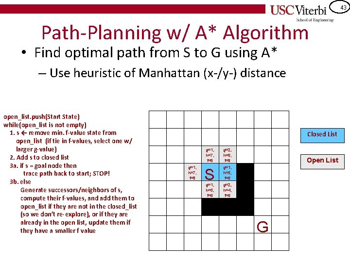
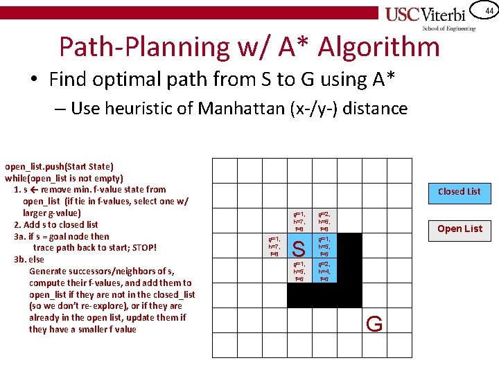
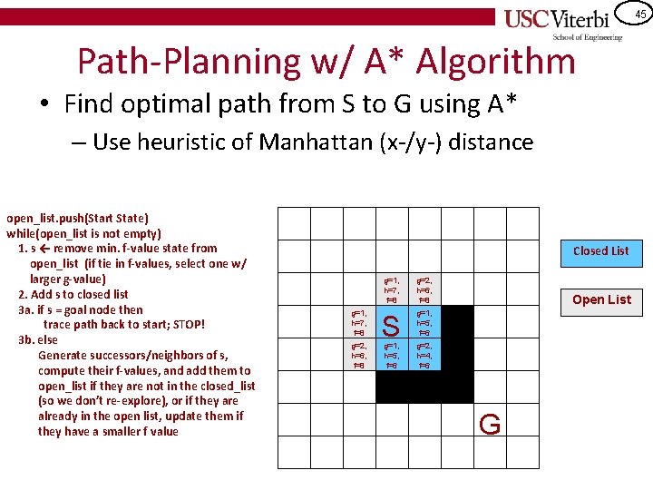
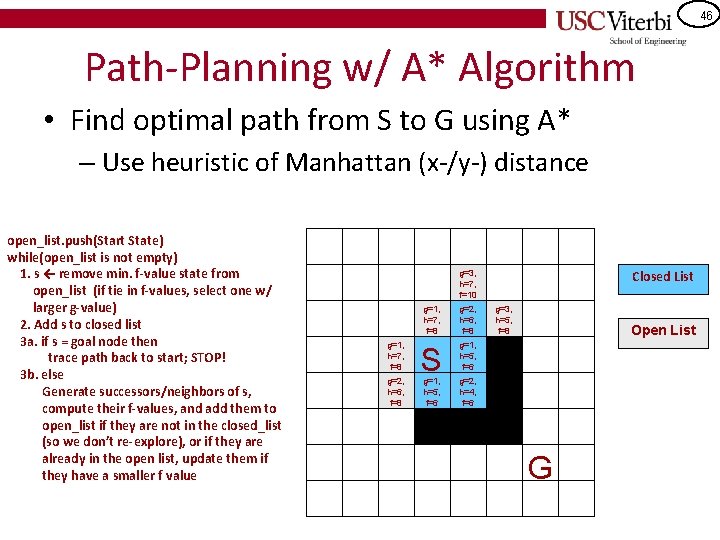
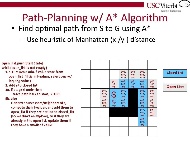
40 Path-Planning w/ A* Algorithm • Find optimal path from S to G using A* – Use heuristic of Manhattan (x-/y-) distance **If implementing this for a programming assignment, please see the slide at the end about alternate closed-list implementation open_list. push(Start State) while(open_list is not empty) 1. s ← remove min. f-value state from open_list (if tie in f-values, select one w/ larger g-value) 2. Add s to closed list 3 a. if s = goal node then trace path back to start; STOP! 3 b. else Generate successors/neighbors of s, compute their f-values, and add them to open_list if they are not in the closed_list (so we don’t re-explore), or if they are already in the open list, update them if they have a smaller f value Closed List Open List S G

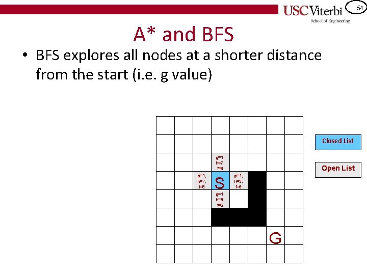
41 Path-Planning w/ A* Algorithm • Find optimal path from S to G using A* – Use heuristic of Manhattan (x-/y-) distance **If implementing this for a programming assignment, please see the slide at the end about alternate closed-list implementation open_list. push(Start State) while(open_list is not empty) 1. s ← remove min. f-value state from open_list (if tie in f-values, select one w/ larger g-value) 2. Add s to closed list 3 a. if s = goal node then trace path back to start; STOP! 3 b. else Generate successors/neighbors of s, compute their f-values, and add them to open_list if they are not in the closed_list (so we don’t re-explore), or if they are already in the open list, update them if they have a smaller f value Closed List Open List g=0, h=6, f=6 S G

42 Path-Planning w/ A* Algorithm • Find optimal path from S to G using A* – Use heuristic of Manhattan (x-/y-) distance open_list. push(Start State) while(open_list is not empty) 1. s ← remove min. f-value state from open_list (if tie in f-values, select one w/ larger g-value) 2. Add s to closed list 3 a. if s = goal node then trace path back to start; STOP! 3 b. else Generate successors/neighbors of s, compute their f-values, and add them to open_list if they are not in the closed_list (so we don’t re-explore), or if they are already in the open list, update them if they have a smaller f value Closed List g=1, h=7, f=8 S Open List g=1, h=5, f=6 G

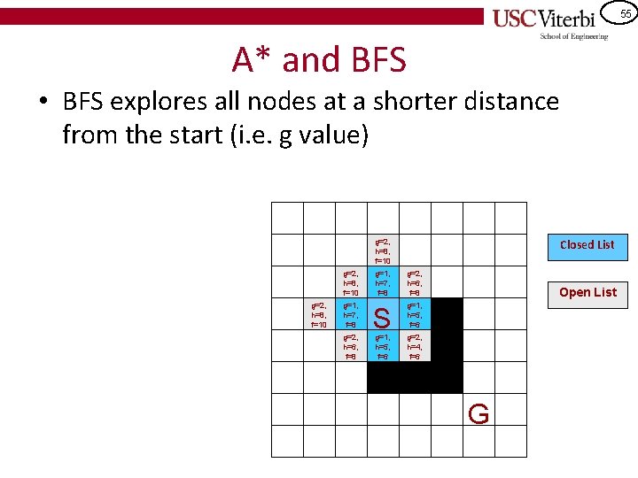
43 Path-Planning w/ A* Algorithm • Find optimal path from S to G using A* – Use heuristic of Manhattan (x-/y-) distance open_list. push(Start State) while(open_list is not empty) 1. s ← remove min. f-value state from open_list (if tie in f-values, select one w/ larger g-value) 2. Add s to closed list 3 a. if s = goal node then trace path back to start; STOP! 3 b. else Generate successors/neighbors of s, compute their f-values, and add them to open_list if they are not in the closed_list (so we don’t re-explore), or if they are already in the open list, update them if they have a smaller f value Closed List g=1, h=7, f=8 g=2, h=6, f=8 S g=1, h=5, f=6 Open List g=2, h=4, f=6 G

44 Path-Planning w/ A* Algorithm • Find optimal path from S to G using A* – Use heuristic of Manhattan (x-/y-) distance open_list. push(Start State) while(open_list is not empty) 1. s ← remove min. f-value state from open_list (if tie in f-values, select one w/ larger g-value) 2. Add s to closed list 3 a. if s = goal node then trace path back to start; STOP! 3 b. else Generate successors/neighbors of s, compute their f-values, and add them to open_list if they are not in the closed_list (so we don’t re-explore), or if they are already in the open list, update them if they have a smaller f value Closed List g=1, h=7, f=8 g=2, h=6, f=8 S g=1, h=5, f=6 Open List g=2, h=4, f=6 G

45 Path-Planning w/ A* Algorithm • Find optimal path from S to G using A* – Use heuristic of Manhattan (x-/y-) distance open_list. push(Start State) while(open_list is not empty) 1. s ← remove min. f-value state from open_list (if tie in f-values, select one w/ larger g-value) 2. Add s to closed list 3 a. if s = goal node then trace path back to start; STOP! 3 b. else Generate successors/neighbors of s, compute their f-values, and add them to open_list if they are not in the closed_list (so we don’t re-explore), or if they are already in the open list, update them if they have a smaller f value Closed List g=1, h=7, f=8 g=2, h=6, f=8 S g=1, h=5, f=6 Open List g=2, h=4, f=6 G

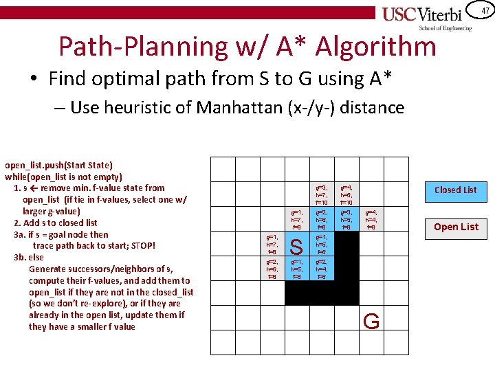
46 Path-Planning w/ A* Algorithm • Find optimal path from S to G using A* – Use heuristic of Manhattan (x-/y-) distance open_list. push(Start State) while(open_list is not empty) 1. s ← remove min. f-value state from open_list (if tie in f-values, select one w/ larger g-value) 2. Add s to closed list 3 a. if s = goal node then trace path back to start; STOP! 3 b. else Generate successors/neighbors of s, compute their f-values, and add them to open_list if they are not in the closed_list (so we don’t re-explore), or if they are already in the open list, update them if they have a smaller f value Closed List g=3, h=7, f=10 g=1, h=7, f=8 g=2, h=6, f=8 S g=1, h=5, f=6 g=3, h=5, f=8 Open List g=2, h=4, f=6 G

47 Path-Planning w/ A* Algorithm • Find optimal path from S to G using A* – Use heuristic of Manhattan (x-/y-) distance open_list. push(Start State) while(open_list is not empty) 1. s ← remove min. f-value state from open_list (if tie in f-values, select one w/ larger g-value) 2. Add s to closed list 3 a. if s = goal node then trace path back to start; STOP! 3 b. else Generate successors/neighbors of s, compute their f-values, and add them to open_list if they are not in the closed_list (so we don’t re-explore), or if they are already in the open list, update them if they have a smaller f value g=2, h=8, f=10 g=1, h=7, f=8 g=3, h=7, f=10 g=2, h=6, f=8 g=2, h=8, f=10 g=3, h=7, f=10 g=4, h=6, f=10 g=1, h=7, f=8 g=2, h=6, f=8 g=3, h=5, f=8 S g=1, h=5, f=6 Closed List g=4, h=4, f=8 g=2, h=4, f=6 g=3, h=5, f=8 G Open List

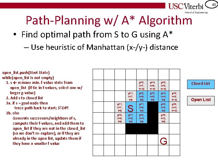
48 Path-Planning w/ A* Algorithm • Find optimal path from S to G using A* – Use heuristic of Manhattan (x-/y-) distance open_list. push(Start State) while(open_list is not empty) 1. s ← remove min. f-value state from open_list (if tie in f-values, select one w/ larger g-value) 2. Add s to closed list 3 a. if s = goal node then trace path back to start; STOP! 3 b. else Generate successors/neighbors of s, compute their f-values, and add them to open_list if they are not in the closed_list (so we don’t re-explore), or if they are already in the open list, update them if they have a smaller f value g=2, h=8, f=10 g=1, h=7, f=8 g=3, h=7, f=10 g=2, h=6, f=8 g=2, h=8, f=10 g=3, h=7, f=10 g=4, h=6, f=10 g=5, h=5, f=10 g=1, h=7, f=8 g=2, h=6, f=8 g=3, h=5, f=8 g=4, h=4, f=8 S g=1, h=5, f=6 g=5, h=3, f=8 g=2, h=4, f=6 g=3, h=5, f=8 G Closed List g=5, h=5, f=10 Open List

49 Path-Planning w/ A* Algorithm • Find optimal path from S to G using A* – Use heuristic of Manhattan (x-/y-) distance open_list. push(Start State) while(open_list is not empty) 1. s ← remove min. f-value state from open_list (if tie in f-values, select one w/ larger g-value) 2. Add s to closed list 3 a. if s = goal node then trace path back to start; STOP! 3 b. else Generate successors/neighbors of s, compute their f-values, and add them to open_list if they are not in the closed_list (so we don’t re-explore), or if they are already in the open list, update them if they have a smaller f value g=2, h=8, f=10 g=1, h=7, f=8 g=3, h=7, f=10 g=2, h=6, f=8 Closed List g=2, h=8, f=10 g=3, h=7, f=10 g=4, h=6, f=10 g=5, h=5, f=10 g=1, h=7, f=8 g=2, h=6, f=8 g=3, h=5, f=8 g=4, h=4, f=8 g=5, h=5, f=10 S g=1, h=5, f=6 g=5, h=3, f=8 g=6, h=4, f=10 g=2, h=4, f=6 g=6, h=2, f=8 g=1, h=5, f=6 g=3, h=5, f=8 G Open List

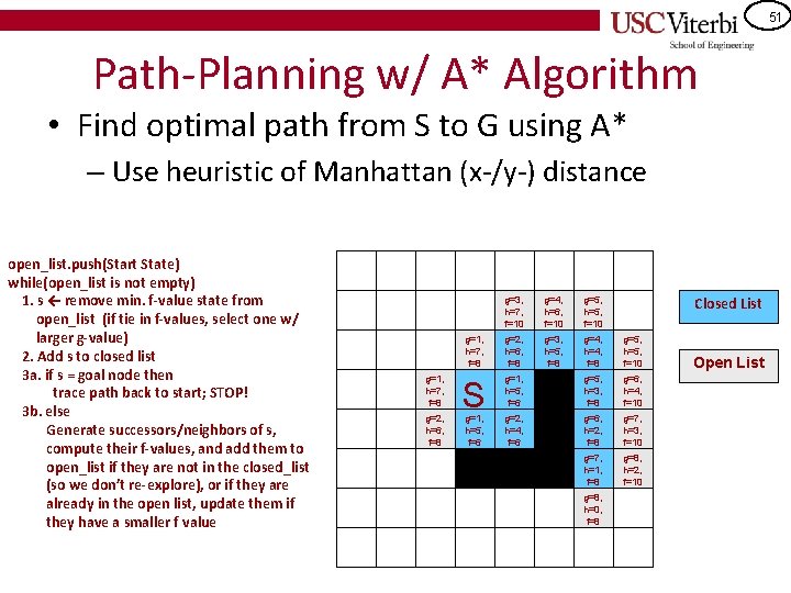
50 Path-Planning w/ A* Algorithm • Find optimal path from S to G using A* – Use heuristic of Manhattan (x-/y-) distance open_list. push(Start State) while(open_list is not empty) 1. s ← remove min. f-value state from open_list (if tie in f-values, select one w/ larger g-value) 2. Add s to closed list 3 a. if s = goal node then trace path back to start; STOP! 3 b. else Generate successors/neighbors of s, compute their f-values, and add them to open_list if they are not in the closed_list (so we don’t re-explore), or if they are already in the open list, update them if they have a smaller f value g=2, h=8, f=10 g=1, h=7, f=8 g=3, h=7, f=10 g=2, h=6, f=8 g=3, h=5, f=8 Closed List g=2, h=8, f=10 g=3, h=7, f=10 g=4, h=6, f=10 g=5, h=5, f=10 g=1, h=7, f=8 g=2, h=6, f=8 g=3, h=5, f=8 g=4, h=4, f=8 g=5, h=5, f=10 S g=1, h=5, f=6 g=5, h=3, f=8 g=6, h=4, f=10 g=2, h=4, f=6 g=6, h=2, f=8 g=7, h=3, f=10 g=1, h=5, f=6 g=7, h=1, f=8 G Open List

51 Path-Planning w/ A* Algorithm • Find optimal path from S to G using A* – Use heuristic of Manhattan (x-/y-) distance open_list. push(Start State) while(open_list is not empty) 1. s ← remove min. f-value state from open_list (if tie in f-values, select one w/ larger g-value) 2. Add s to closed list 3 a. if s = goal node then trace path back to start; STOP! 3 b. else Generate successors/neighbors of s, compute their f-values, and add them to open_list if they are not in the closed_list (so we don’t re-explore), or if they are already in the open list, update them if they have a smaller f value g=2, h=8, f=10 g=1, h=7, f=8 g=3, h=7, f=10 g=2, h=6, f=8 g=3, h=5, f=8 Closed List g=2, h=8, f=10 g=3, h=7, f=10 g=4, h=6, f=10 g=5, h=5, f=10 g=1, h=7, f=8 g=2, h=6, f=8 g=3, h=5, f=8 g=4, h=4, f=8 g=5, h=5, f=10 S g=1, h=5, f=6 g=5, h=3, f=8 g=6, h=4, f=10 g=2, h=4, f=6 g=6, h=2, f=8 g=7, h=3, f=10 g=7, h=1, f=8 g=8, h=2, f=10 g=1, h=5, f=6 g=8, h=0, f=8 G Open List

52 Path-Planning w/ A* Algorithm • Find optimal path from S to G using A* – Use heuristic of Manhattan (x-/y-) distance open_list. push(Start State) while(open_list is not empty) 1. s ← remove min. f-value state from open_list (if tie in f-values, select one w/ larger g-value) 2. Add s to closed list 3 a. if s = goal node then trace path back to start; STOP! 3 b. else Generate successors/neighbors of s, compute their f-values, and add them to open_list if they are not in the closed_list (so we don’t re-explore), or if they are already in the open list, update them if they have a smaller f value g=2, h=8, f=10 g=1, h=7, f=8 g=3, h=7, f=10 g=2, h=6, f=8 g=3, h=5, f=8 Closed List g=2, h=8, f=10 g=3, h=7, f=10 g=4, h=6, f=10 g=5, h=5, f=10 g=1, h=7, f=8 g=2, h=6, f=8 g=3, h=5, f=8 g=4, h=4, f=8 g=5, h=5, f=10 S g=1, h=5, f=6 g=5, h=3, f=8 g=6, h=4, f=10 g=2, h=4, f=6 g=6, h=2, f=8 g=7, h=3, f=10 g=7, h=1, f=8 g=8, h=2, f=10 g=1, h=5, f=6 g=8, h=0, f=8 G Open List

53 Path-Planning w/ A* Algorithm • Find optimal path from S to G using A* – Use heuristic of Manhattan (x-/y-) distance open_list. push(Start State) while(open_list is not empty) 1. s ← remove min. f-value state from open_list (if tie in f-values, select one w/ larger g-value) 2. Add s to closed list 3 a. if s = goal node then trace path back to start; STOP! 3 b. else Generate successors/neighbors of s, compute their f-values, and add them to open_list if they are not in the closed_list (so we don’t re-explore), or if they are already in the open list, update them if they have a smaller f value g=2, h=8, f=10 g=1, h=7, f=8 g=3, h=7, f=10 g=2, h=6, f=8 g=3, h=5, f=8 Closed List g=2, h=8, f=10 g=3, h=7, f=10 g=4, h=6, f=10 g=5, h=5, f=10 g=1, h=7, f=8 g=2, h=6, f=8 g=3, h=5, f=8 g=4, h=4, f=8 g=5, h=5, f=10 S g=1, h=5, f=6 g=5, h=3, f=8 g=6, h=4, f=10 g=2, h=4, f=6 g=6, h=2, f=8 g=7, h=3, f=10 g=7, h=1, f=8 g=8, h=2, f=10 g=1, h=5, f=6 g=8, h=0, f=8 G Open List

54 A* and BFS • BFS explores all nodes at a shorter distance from the start (i. e. g value) Closed List g=1, h=7, f=8 S Open List g=1, h=5, f=6 G

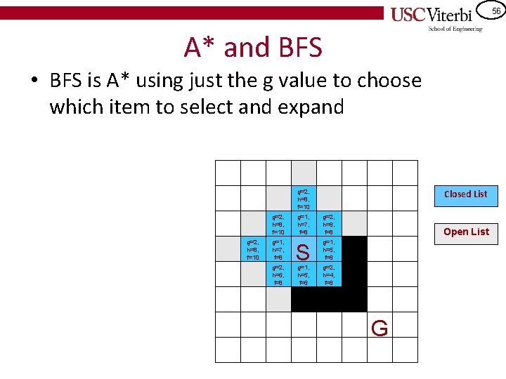
55 A* and BFS • BFS explores all nodes at a shorter distance from the start (i. e. g value) Closed List g=2, h=8, f=10 g=1, h=7, f=8 g=2, h=6, f=8 S g=1, h=5, f=6 Open List g=2, h=4, f=6 G

56 A* and BFS • BFS is A* using just the g value to choose which item to select and expand Closed List g=2, h=8, f=10 g=1, h=7, f=8 g=2, h=6, f=8 S g=1, h=5, f=6 Open List g=2, h=4, f=6 G

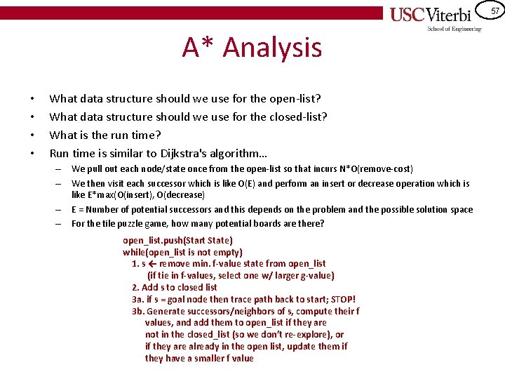
57 A* Analysis • • What data structure should we use for the open-list? What data structure should we use for the closed-list? What is the run time? Run time is similar to Dijkstra's algorithm… – We pull out each node/state once from the open-list so that incurs N*O(remove-cost) – We then visit each successor which is like O(E) and perform an insert or decrease operation which is like E*max(O(insert), O(decrease) – E = Number of potential successors and this depends on the problem and the possible solution space – For the tile puzzle game, how many potential boards are there? open_list. push(Start State) while(open_list is not empty) 1. s ← remove min. f-value state from open_list (if tie in f-values, select one w/ larger g-value) 2. Add s to closed list 3 a. if s = goal node then trace path back to start; STOP! 3 b. Generate successors/neighbors of s, compute their f values, and add them to open_list if they are not in the closed_list (so we don’t re-explore), or if they are already in the open list, update them if they have a smaller f value

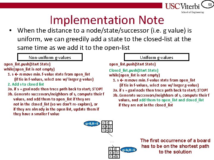
58 Implementation Note • When the distance to a node/state/successor (i. e. g value) is uniform, we can greedily add a state to the closed-list at the same time as we add it to the open-list Uniform g-values Non-uniform g-values open_list. push(Start State) while(open_list is not empty) 1. s ← remove min. f-value state from open_list (if tie in f-values, select one w/ larger g-value) 2. Add s to closed list 3 a. if s = goal node then trace path back to start; STOP! 3 b. Generate successors/neighbors of s, compute their f values, and add them to open_list if they are not in the closed_list (so we don’t re-explore), or if they are already in the open list, update them if they have a smaller f value g=0, H=6 open_list. push(Start State) Closed_list. push(Start State) while(open_list is not empty) 1. s ← remove min. f-value state from open_list (if tie in f-values, select one w/ larger g-value) 3 a. if s = goal node then trace path back to start; STOP! 3 b. Generate successors/neighbors of s, compute their f values, and add them to open_list and closed_list if they are not in the closed_list 1 2 4 8 3 7 6 5 … 1 2 4 8 3 7 6 5 g=k, H=6 The first occurrence of a board has to be on the shortest path to the solution

59 BETWEENESS CENTRALITY

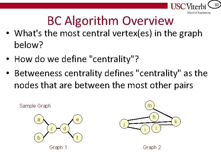
60 BC Algorithm Overview • What's the most central vertex(es) in the graph below? • How do we define "centrality"? • Betweeness centrality defines "centrality" as the nodes that are between the most other pairs m Sample Graph a e c d b h j i k l f Graph 1 Graph 2

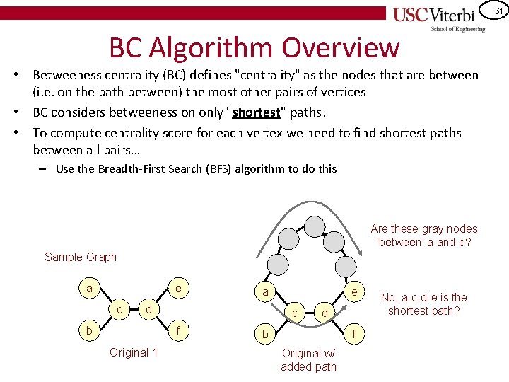
61 BC Algorithm Overview • Betweeness centrality (BC) defines "centrality" as the nodes that are between (i. e. on the path between) the most other pairs of vertices • BC considers betweeness on only "shortest" paths! • To compute centrality score for each vertex we need to find shortest paths between all pairs… – Use the Breadth-First Search (BFS) algorithm to do this Are these gray nodes 'between' a and e? Sample Graph a e c a d b c f Original 1 e d b f Original w/ added path No, a-c-d-e is the shortest path?

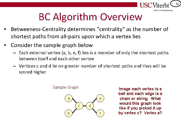
62 BC Algorithm Overview • Betweeness-Centrality determines "centrality" as the number of shortest paths from all-pairs upon which a vertex lies • Consider the sample graph below – Each external vertex (a, b, e, f) lies is a member of only the shortest paths between itself and each other vertex – Vertices c and d lie on greater number of shortest paths and thus will be scored higher Sample Graph a e c b d f Image each vertex is a ball and each edge is a chain or string. What would this graph look like if you picked it up by vertex c? Vertex a?

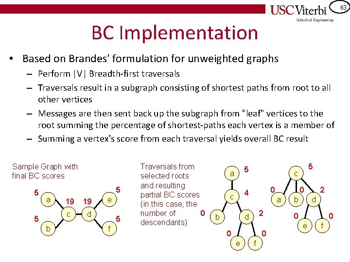
63 BC Implementation • Based on Brandes' formulation for unweighted graphs – Perform |V| Breadth-first traversals – Traversals result in a subgraph consisting of shortest paths from root to all other vertices – Messages are then sent back up the subgraph from "leaf" vertices to the root summing the percentage of shortest-paths each vertex is a member of – Summing a vertex's score from each traversal yields overall BC result Sample Graph with final BC scores 5 5 a 5 b 19 19 c d e 5 f Traversals from selected roots and resulting partial BC scores (in this case, the 0 number of descendants) a 5 c 4 b 0 0 a 2 d 0 0 e 5 c f b 2 d 0 0 e f

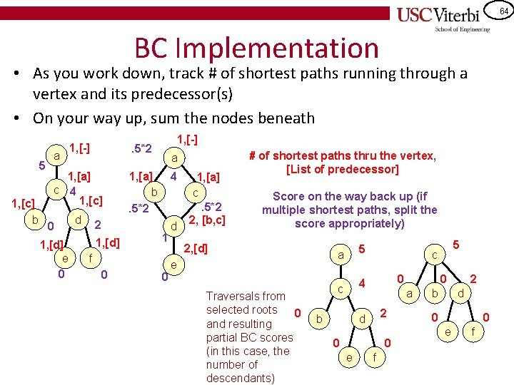
64 BC Implementation • As you work down, track # of shortest paths running through a vertex and its predecessor(s) • On your way up, sum the nodes beneath 5 1, [c] b 1, [-] . 5*2 1, [a] c 4 1, [c] 1, [a] b. 5*2 a 0 1, [d] e 0 d 2 1, [d] 1, [-] a 4 1 f 0 0 d 1, [a] c. 5*2 2, [b, c] # of shortest paths thru the vertex, [List of predecessor] Score on the way back up (if multiple shortest paths, split the score appropriately) 2, [d] e Traversals from selected roots 0 and resulting partial BC scores (in this case, the number of descendants) a 5 c 4 b 0 0 a 2 d 0 0 e 5 c f b 2 d 0 0 e f