1 Circular Flow of Economic Activity Graphical visual

1. Circular Flow of Economic Activity- Graphical (visual) way of showing how productive resources, money, and goods and services flow between individuals (households), firms (businesses), government and international sector.

2. Resource/ Factor Market- Market where productive resources are exchanged for $. 3. Product Market- Market where money is exchanged for goods and services.

Circular Flow Diagram Resource Market Businesses Households Product Market

Resource Market Resources- $ Income/ Costs 1. Natural- Rent 2. Human- Wages, Salaries, Tips Commissions 3. Capital- Interest 4. Households Entrepreneurship- Profit Businesses Product Market Injections ($) 1. Government Spending 2. Exports 3. Investment Withdrawals ($) Circular Flow of Economic Activity 1. Taxes 2. Imports 3. Savings

Both Flows Are Equal Resource Market Businesses Households Product Market

3 Withdrawals of $ from the Flow 1. Taxes 2. Imports 3. Savings 3 Injections of $ into the Flow 1. Government Spending 2. Exports 3. Investment

International Sector Exports $ ey n o M $ Households G & S $ Government Productive R $ Mo ne y G&S PR M Imports Product Market S G & Fin Mkt Savings $ G & S Investment G & S Businesses $ Productive Resources on e y Resource Market M ey n o

4. Demand- The desire plus the ability and willingness to pay. 5. Demand Schedule- A chart showing the quantity demanded at different prices at a given point in time. Ex: Compact discs Price 6. Law of Demand- Demand for a product varies inversely with its price. More will be demanded at a lower price than at a higher price (Thumbs different). D 0 Quantity

Individual Demand P 6 P Qd $5 10 4 20 3 35 2 55 1 80 5 Price (per bushel) Individual Demand 4 3 2 1 0 D 10 20 30 40 50 60 70 80 Quantity Demanded (bushels per week) Q

Price 7. Change in the quantity demanded (∆Qd)- The change in the amount purchased in response to the change in price(movement along the demand curve). P 1 ∆Qd ∆Q d P 0 D 0 0 Price 8. Change in Demand (∆D)- A shift in the entire demand curve. Caused by changing conditions other than price! Q 1 Q 0 Quantity ∆D D 1 D 2 D 0 0 Quantity

Demand Can Increase or Decrease P 6 P Qd $5 10 4 20 3 35 2 55 1 80 5 Price (per bushel) Individual Demand Increase in Demand 4 3 2 1 0 D 2 Decrease in Demand 2 4 6 8 10 D 1 D 3 12 14 16 18 Q Quantity Demanded (bushels per week)

Demand Can Increase or Decrease An Increase in Demand Means a Movement of the Line P 6 P Qd $5 10 4 20 3 35 2 55 1 80 A Movement Between Any Two Points on a Demand Curve is Called a Change in Quantity Demanded 5 Price (per bushel) Individual Demand 4 3 2 1 0 D 2 Decrease in Demand 2 4 6 8 10 D 1 D 3 12 14 16 18 Q Quantity Demanded (bushels per week)

9. Supply- The quantity of a product that would be produced and offered for sale at each and every possible price. 10. Supply Schedule- A chart showing the quantity produced at each and every possible price in the market. Ex: Yard Work Price 11. Law of Supply- The quantity of a product offered for sale varies directly with price. More will be supplied at a higher price than at a lower price (Thumbs same). S 0 Quantity

Individual Supply P 6 P Qs $5 60 4 50 3 35 2 20 1 5 S 1 5 Price (per bushel) Individual Supply 4 3 2 1 0 10 20 30 40 50 60 70 Quantity Supplied (bushels per week) Q

Price 12. Change in the Quantity Supplied (∆Qs)- The change in the amount of a product offered for sale (supplied) because of a price change. Movement along the supply curve. S P 1 s ∆Q ∆QS P 0 0 Price Q 0 Q 1 Quantity S 2 S 0 S 1 13. Change in Supply (∆S)- A shift in the entire supply curve. Caused by changing conditions other than price! ∆S 0 Quantity

Supply Can Increase or Decrease P 6 P Qs $5 60 4 50 3 35 2 20 1 5 5 Price (per bushel) Individual Supply S 3 S 1 S 2 4 3 2 1 0 2 4 6 8 10 12 14 Quantity Supplied (bushels per week) Q

Supply Can Increase or Decrease A Movement Between Any Two Points on a Supply Curve is Called a 5 Change in Quantity Supplied P Individual Supply P Qs $5 60 4 50 3 35 2 20 1 5 Price (per bushel) 6 S 3 S 1 S 2 4 3 2 An Increase in Supply Means a Movement of the Line 1 0 2 4 6 8 10 12 14 Quantity Supplied (bushels per week) Q

Elasticity Notes 14. Price Elasticity of Demand- The extent to which changes in price cause changes in the quantity demanded.

15. Elastic Demand- A change in price leads to a relatively large change in quantity demanded. Ex: Ice Cream, Disneyland Vacation Price ∆Q d P 1 P 0 D 0 Quantity Price P 1 ∆Q Looks like an “I” d 16. Inelastic Demand- A change in price leads to a relatively small change in quantity demanded. Ex: Gasoline, Cigarettes Q 0 Q 1 P 0 D 0 Q 1 Q 0 Quantity

Elasticity Notes 15. Products that have elastic demand curves have these characteristics: Ex: Ice Cream, Disneyland Vacation 1. Many Substitutes 2. Luxuries 3. Relatively Expensive

Elasticity Notes 16. Products that have inelastic demand curves have these characteristics: 1. Few Substitutes Ex: Gasoline, Cigarettes 2. Necessities 3. Relatively Inexpensive

Extreme Cases Perfectly Inelastic Demand P D 1 Perfectly Inelastic Demand (Ed = 0) 0 Q Perfectly Elastic Demand P 0 Perfectly Elastic Demand (Ed = ∞) D 2 Q

Elasticity Notes 17. Time and Price Elasticity of Demand- As time goes on more substitutes become available and the product becomes less necessary. Therefore, as time goes on the more elastic the product becomes.

Elasticity Notes 18. Price Elasticity of Supply- The extent to which changes in price cause changes in the quantity supplied.

Price Q 1 Quantity Q 0 Price S P 1 s Ex: Sports car, Space Shuttle, Oil, Gold ∆Qs P 0 0 20. Inelastic Supply- A change in price leads to a relatively small change in quantity supplied. S P 1 P 0 0 ∆Q 19. Elastic Supply- A change in price leads to a relatively large change in quantity supplied. Ex: Fast Food, T-Shirts Q 0 Q 1 Looks like an “I” Quantity

Elasticity Notes 19. Products that have elastic supply curves have these characteristics: Ex: Fast Food, T-Shirts 1. Low technology 2. Easy to find or produce 3. Few skills needed

Elasticity Notes 20. Products that have inelastic supply curves have these characteristics: Ex: Sports car, Space Shuttle, Oil, Gold 1. High technology 2. Difficult to find or produce 3. Skilled workers needed

Price Elasticity of Supply n Applications n Antiques/ Original Art and Reproductions With originals it’s hard /impossible to make more n With Reproductions you can mass produce them quickly n n Gold Prices- Boom and Bust cycles Gold Prices have shot up so can gold mines produce a lot more gold quickly? n The fastest way to produce more gold has been to do what? n Think about all of the “We Buy Gold! “ signs around town… n Get people, mostly women, to sell their old jewelry n There are even “gold parties” where women gather to have fun and sell their old gold jewelry that they don’t wear any more. n

Elasticity Notes 21. Time and Price Elasticity of Supply- As time goes on more technology and more capital become available and productivity increases. Therefore, as time goes on the more elastic the product becomes.

Marginal Utility Notes 22. Marginal Utility- The extra utility or satisfaction a person gets from acquiring an additional "unit" of a product. Amount added "at the margin". 23. Principle of Diminishing Marginal Utility- Each additional unit of a product will be less satisfying than the previous one. The more of a product a person acquires, the less likely they will consume (purchase) more. Ex: Candy consumption, Buying in bulk (Costco, Sam’s Club, Buying a case of soda instead of a can

24. Market Price- The price where quantity supplied equals quantity demanded (Qs = Qd). Occurs at the intersection of the supply and demand curves. Also known as equilibrium price and market clearing price. Price S Qs = Qd P 0 D 0 Quantity 3 Names for the intersection point: 1. Market Price 2. Equilibrium (Price) 3. Market-Clearing Price

Market Equilibrium 200 Buyers & 200 Sellers Market Demand 200 Buyers Qd $5 2, 000 4 4, 000 3 7, 000 2 11, 000 1 6 16, 000 S 5 Price (per bushel) P Market Supply 200 Sellers 4 3 2 1 0 D 2 4 6 7 8 10 12 14 16 18 Bushels of Corn (thousands per week) P Qs $5 12, 000 4 10, 000 3 7, 000 2 4, 000 1 1, 000

Determinants of Demand Supply 25. Determinants of Demand: Reasons for Change/ Shift in Demand (SEPTIC); A change in: Price of Substitutes- things that replace each other: pork v. beef, pinto beans vs. black beans, TV shows and video rentals (If P of Substitute ↑, D for other good ↑) (If P of A ↑, D for B ↑). vs.

25. Determinants of Demand: Reasons for Change/ Shift in Demand (SEPTIC); A change in: Consumer Expectations-if they expect a change in prices or their income to happen in the future or a prediction is made

25. Determinants of Demand: Reasons for Change/ Shift in Demand (SEPTIC); A change in: Population: Number of consumers, more or less people means more or less demand

25. Determinants of Demand: Reasons for Change/ Shift in Demand (SEPTIC); A change in: Consumer Taste- preferences, styles, fads, fashion, health, advertising, popularity

25. Determinants of Demand: Reasons for Change/ Shift in Demand (SEPTIC); A change in: Income (y) (If Y ↑ , D ↑. If Y↓, D↓) more or less income means more or less demand. Ex: Steak, Sports Car

25. Determinants of Demand: Reasons for Change/ Shift in Demand (SEPTIC); A change in: Price of Complementary good- things that go together: ketchup and fries; movies and popcorn, cars and gasoline (If P of Complement ↑, D for other good ↓) (If P of A ↑, D for B ↓).

26. Determinants of Supply: Reasons for Change/ Shift in Supply (GETNo. Credit); A change in: Government Policies - taxes, regulations, tariffs, quotas, setting prices, or any other government action.

26. Determinants of Supply: Reasons for Change/ Shift in Supply (GETNo. Credit); A change in: Expectations- businesses expect a change to occur to sales, profits, etc. in the future.

26. Determinants of Supply: Reasons for Change/ Shift in Supply (GETNo. Credit); A change in: Technology- increases the efficiency of your natural, human, capital, and entrepreneurship resources.

26. Determinants of Supply: Reasons for Change/ Shift in Supply (GETNo. Credit); A change in: Number of Suppliers- Companies entering or leaving the market.

26. Determinants of Supply: Reasons for Change/ Shift in Supply (GETNo. Credit); A change in: Costs of Production- anything that increases or decreases the cost of your land, labor, capital, and entrepreneurship.

27. The 4 shifts of the Supply and Demand Curve Shift 1 - Demand Away Price (P) S 4. ∆QS; Movement along the S curve. P 1 5. Price ↑ from P 0 to P 1. P 0 5. Quantity ↑ from Q 0 to Q 1. D 1 D 0 0 Q 1 Quantity (Q)

27. The 4 shifts of the Supply and Demand Curve Shift 2 - Demand Towards Price (P) S 4. ∆QS; Movement along the S curve. 5. Price ↓ from P 0 to P 1. P 0 P 1 D 1 0 Q 1 Q 0 D 0 5. Quantity ↓ from Q 0 to Q 1. Quantity (Q)

27. The 4 shifts of the Supply and Demand Curve Shift 3 - Supply Away Price (P) S 0 4. ∆Qd; S 1 Movement along the D curve. 5. Price ↓ from P 0 to P 1. P 0 P 1 D 0 0 Q 1 Quantity (Q) 5. Quantity ↑ from Q 0 to Q 1.

27. The 4 shifts of the Supply and Demand Curve Shift 4 - Supply Towards S 1 Price (P) S 0 P 1 5. Price ↑ from P 0 to P 1. P 0 D 0 0 4. ∆Qd; Movement along the D curve. Q 1 Q 0 5. Quantity ↓ from Q 0 to Q 1. Quantity (Q)

28. Price Floor- Legislated or regulated minimum price below which transactions (buying or selling) are prohibited. Will cause a surplus (Qs › Qd). Done for Producers! 29. Price Ceiling- Legislated or regulated maximum price above which transactions (buying or selling) are prohibited (Qd › Qs). Will cause a shortage. To get around this producers and consumers will create a black market. Done for consumers! Price Floor on the TOP! S Pf P 0 D 0 Price Qd Q 0 Qs Quantity Ceiling on the BOTTOM! S P 0 Pc D 0 Qs Q 0 Qd Quantity

Floors and Ceilings When the government sets the price 200 Buyers & 200 Sellers Market Demand 200 Buyers Qd $5 2, 000 4 4, 000 3 7, 000 2 11, 000 1 6 16, 000 Bushel Surplus 5 Price (per bushel) P Market Supply 200 Sellers S P Qs $5 12, 000 4 10, 000 3 7, 000 $2 Price Ceiling 2 4, 000 1 1, 000 $4 Price Floor 4 3 2 7, 000 Bushel Shortage 1 0 2 4 6 7 8 10 D 12 14 16 18 Bushels of Corn (thousands per week)

Government-Set Prices n Price Ceilings on Gasoline n n Rationing Problem Black Markets Rent Controls n Price Floors on Wheat n Optimal Allocation of Resources n 3. 2

Why is it that some industries have a small number of business firms that dominate the industry and other industries have many firms with no one firm that dominates? Economists have been able to classify different industries into 4 broad categories or structures based on how much competition there is in an industry:

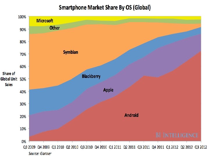
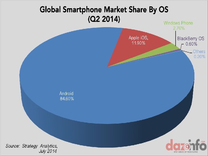
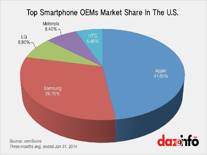
United States only

(2011)

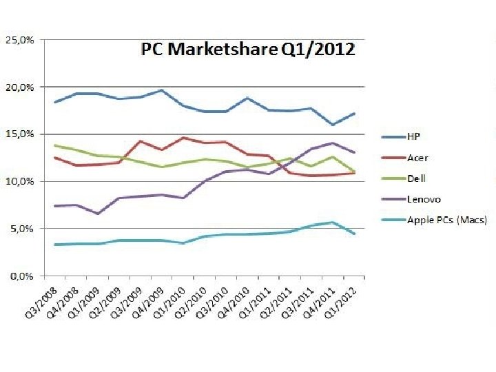
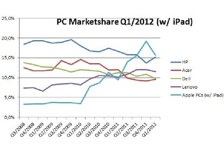
US Auto Market Share

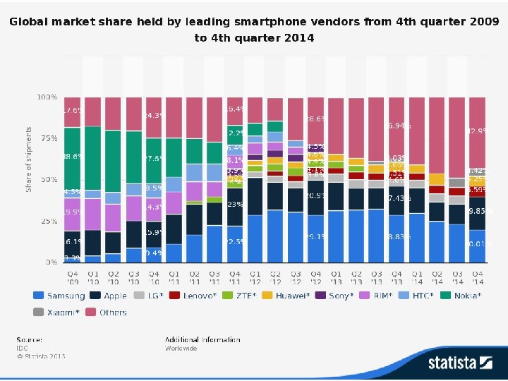
2011 TV Global Market Share

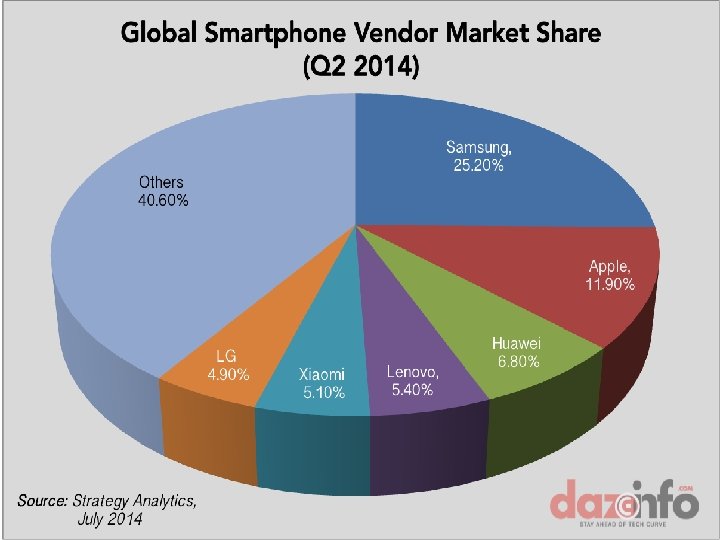
August 2014

Spectrum of Market Structures MOST COMPETITIVE--------------LEAST COMPETITIVE 100%/ Total Competition--------------0%/No Competition Number of firms in the industry Perfect Competition Monopolistic Competition 1. Many Buyers and Sellers Oligopoly Monopoly 1. A few 1. One firms seller dominates the industry

Spectrum of Market Structures MOST COMPETITIVE--------------LEAST COMPETITIVE 100%/ Total Competition--------------0%/No Competition Type of Product Sold Perfect Competition Monopolistic Competition Oligopoly Monopoly 2. Slightly 2. Very 2. Unique/ One 2. Homogeneous Differentiated of a kind / Same/ Identical

Spectrum of Market Structures MOST COMPETITIVE--------------LEAST COMPETITIVE 100%/ Total Competition--------------0%/No Competition Ease of Entry and Exit from the Industry Perfect Competition Monopolistic Competition 3. Easiest 3. Easy Oligopoly Monopoly 3. Difficult 3. Entry can be because of high blocked by cost of capital government or marketing protections costs

Spectrum of Market Structures MOST COMPETITIVE--------------LEAST COMPETITIVE 100%/ Total Competition--------------0%/No Competition Perfect Competition Monopolistic Competition Oligopoly Monopoly Control firms have over the price they charge 4. None; firms must accept the market price 4. A little; firms can charge more for a special service or feature they might have 4. A lot; price can be set higher than other nondifferentiated products 4. Complete; business is a “price setter” at the price where profits are maximized

Spectrum of Market Structures MOST COMPETITIVE--------------LEAST COMPETITIVE 100%/ Total Competition--------------0%/No Competition Perfect Competition Monopolistic Competition Non-price 5. None, all of 5. A little; competition/ firms offer the products product special are the same differentiation- services or competition features they based on things might have other than price but most can (ads, brand be easily names, color, copied taste, quality, features, packaging, etc. ) Oligopoly Monopoly 5. A lot; large amounts of advertising; emphasis on branding, design, style, quality, etc. 5. Little or none since entry can be controlled; ads focus on building goodwill towards the company or product superiority

Banking consolidation/ mergers creates an oligopoly dominated by 4 banks: Citigroup, JPMorgan Chase, Bof. A, and Wells Fargo

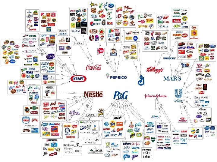
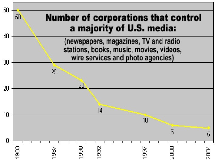
Media Family Tree: Top 15 Media Companies

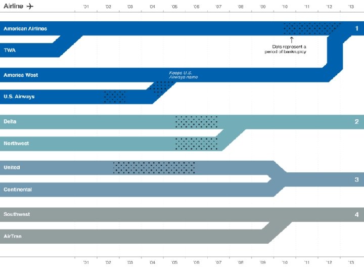
Spectrum of Market Structures MOST COMPETITIVE--------------LEAST COMPETITIVE 100%/ Total Competition--------------0%/No Competition Examples Perfect Competition Grain farming Monopolistic Competition Doctors, Lawyers, Dry Cleaning, Real Estate Agents, Sit down restaurants, Fruits and Vegetables, Oligopoly Monopoly Soda, Beer, Airlines, Fast Food, Soap, Shampoo Computers, Cereal, Groceries, Coffee, Diapers, Entertainment, Banking 4 types of legal monopolies; allowed by government b/c they benefit society in some way 1. Patents 2. Copyrights 3. Trademarks 4. Public Utilities- Electricity, Cable, Nat Gas, Phone, H 2 O

Total Revenue Test- If Price (P) ↑ and Total Revenue (TR) ↓ , then Elastic; If Price (P) ↑ and Total Revenue (TR) ↑ , then Inelastic. Why? Price ∆Q d P 1 Price Effect P 0 Q 1 Q 0 D 0 Quantity Price Effect- Increase in P of the ONE item increases TR Elastic products: Quantity effect is greater than Price effect Q Effect Quantity Effect 0 Price Effect d ∆Q P 1 0 Q 1 Q 0 D 0 Quantity Effect- Increase in P reduces the # of units sold and decreases TR Inelastic products: Price effect is greater than Quantity effect

The Total Revenue Test W 18. 2 Total Revenue (TR) TR = P x Q Elastic Demand n P $3 a 2 1 b D 1 0 10 20 30 40 Q

The Total Revenue Test Total Revenue (TR) TR = P x Q Inelastic Demand n P c $4 3 2 d 1 D 2 0 10 20 Q W 18. 2

The Total Revenue Test W 18. 2 Total Revenue (TR) TR = P x Q Unit-Elastic n P e $3 2 f 1 D 3 0 10 20 30 Q