1 Chapter 3 Nodal and loop analysis techniques

1 Chapter 3. Nodal and loop analysis techniques EMLAB

Contents 2 1. Nodal analysis 2. Loop analysis 3. Application examples 4. Design examples EMLAB

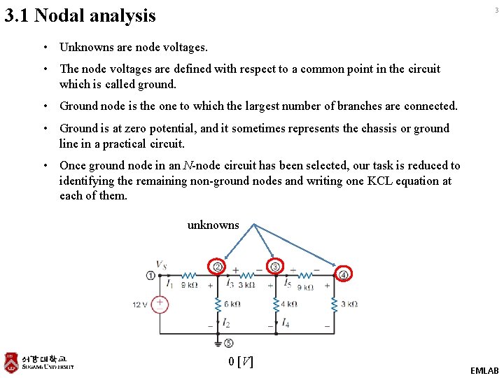
3. 1 Nodal analysis 3 • Unknowns are node voltages. • The node voltages are defined with respect to a common point in the circuit which is called ground. • Ground node is the one to which the largest number of branches are connected. • Ground is at zero potential, and it sometimes represents the chassis or ground line in a practical circuit. • Once ground node in an N-node circuit has been selected, our task is reduced to identifying the remaining non-ground nodes and writing one KCL equation at each of them. unknowns 0 [V] EMLAB

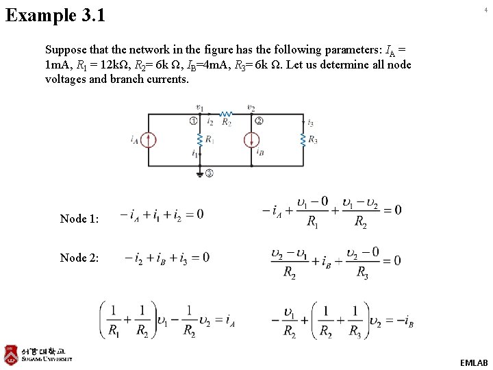
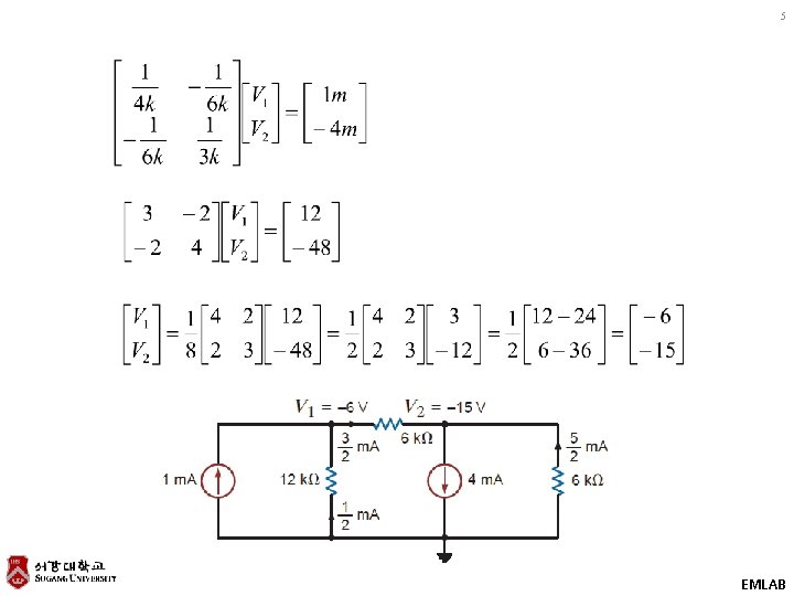
Example 3. 1 4 Suppose that the network in the figure has the following parameters: IA = 1 m. A, R 1 = 12 kΩ, R 2= 6 k Ω, IB=4 m. A, R 3= 6 k Ω. Let us determine all node voltages and branch currents. Node 1: Node 2: EMLAB

5 EMLAB

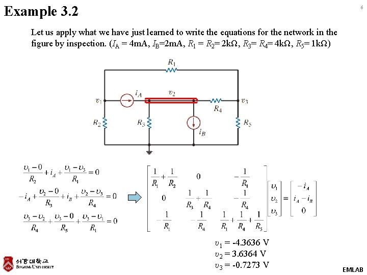
Example 3. 2 6 Let us apply what we have just learned to write the equations for the network in the figure by inspection. (IA = 4 m. A, IB=2 m. A, R 1 = R 2= 2 kΩ, R 3= R 4= 4 kΩ, R 5= 1 kΩ) υ1 = -4. 3636 V υ2 = 3. 6364 V υ3 = -0. 7273 V EMLAB

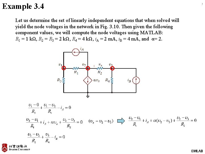
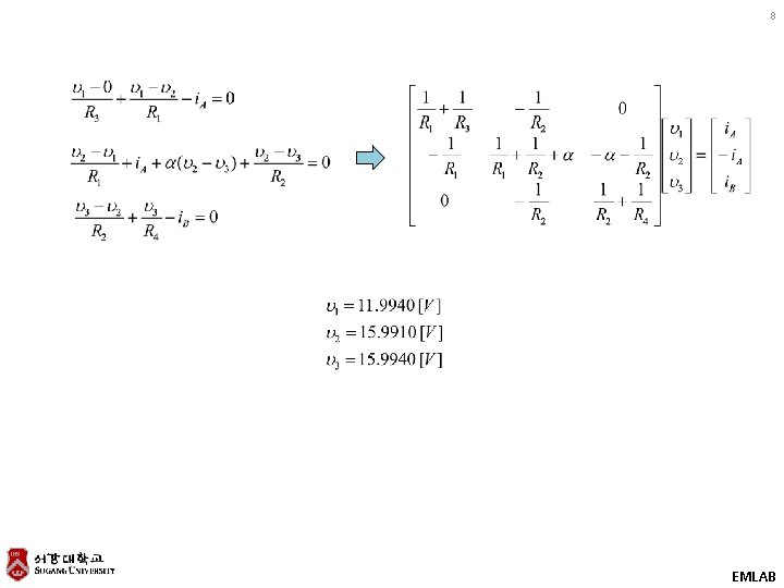
Example 3. 4 7 Let us determine the set of linearly independent equations that when solved will yield the node voltages in the network in Fig. 3. 10. Then given the following component values, we will compute the node voltages using MATLAB: R 1 = 1 kΩ, R 2 = R 3 = 2 kΩ, R 4 = 4 kΩ, i. A = 2 m. A, i. B = 4 m. A, and α= 2. EMLAB

8 EMLAB

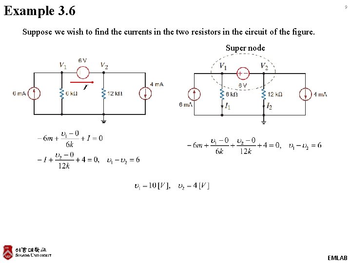
Example 3. 6 9 Suppose we wish to find the currents in the two resistors in the circuit of the figure. Super node EMLAB

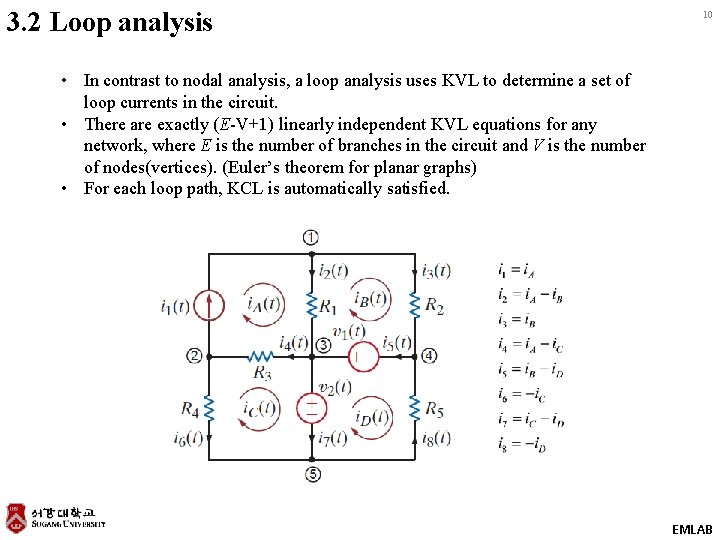
3. 2 Loop analysis 10 • In contrast to nodal analysis, a loop analysis uses KVL to determine a set of loop currents in the circuit. • There are exactly (E-V+1) linearly independent KVL equations for any network, where E is the number of branches in the circuit and V is the number of nodes(vertices). (Euler’s theorem for planar graphs) • For each loop path, KCL is automatically satisfied. EMLAB

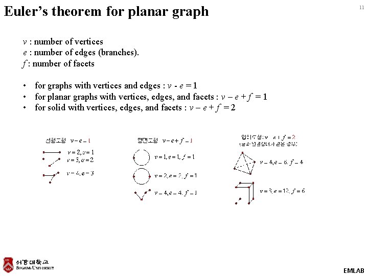
Euler’s theorem for planar graph 11 v : number of vertices e : number of edges (branches). f : number of facets • for graphs with vertices and edges : v - e = 1 • for planar graphs with vertices, edges, and facets : v – e + f = 1 • for solid with vertices, edges, and facets : v – e + f = 2 EMLAB

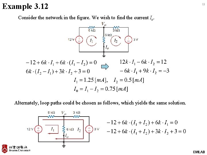
Example 3. 12 12 Consider the network in the figure. We wish to find the current Io. Alternately, loop paths could be chosen as follows, which yields the same solution. EMLAB

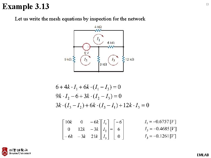
Example 3. 13 13 Let us write the mesh equations by inspection for the network EMLAB

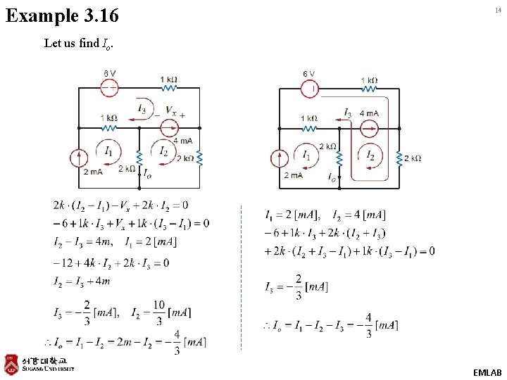
Example 3. 16 14 Let us find Io. EMLAB

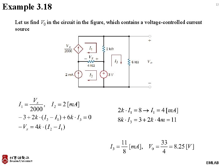
Example 3. 18 15 Let us find V 0 in the circuit in the figure, which contains a voltage-controlled current source EMLAB

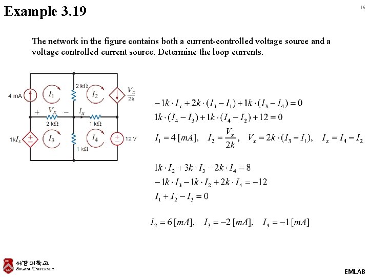
Example 3. 19 16 The network in the figure contains both a current-controlled voltage source and a voltage controlled current source. Determine the loop currents. EMLAB

Some Matlab command 17 A= [2, 3, 1; 4, 5, 7] A= [1: 2: 9] A= A’ A= A-1 EMLAB

18 EMLAB