1 Chapter 3 Introduction to Predictive Modeling From

1 Chapter 3 Introduction to Predictive Modeling : From Correlation to Supervised Segmentation 建立預測模型 --- 從關連到監督式區隔

2 Fundamental concepts: 基本觀念 Identifying informative attributes; Segmenting data by progressive attribute selection. 找出具傳遞訊息能力變數、藉逐步選擇變數將資 料區隔 Exemplary techniques: 示範性技術 Finding correlations; Attribute/variable selection; Tree induction. 找 出相關性、屬性/變數的選擇、決策樹歸納法

3 The previous chapters discussed models and modeling at a high level. This chapter delves into one of the main topics of data mining: predictive modeling. 前面兩章講到模型，本章 將深入資料探勘的主要議題 --- 建立預測的模型 Following our example of data mining for churn prediction from the first section, we will begin by thinking of predictive modeling as supervised segmentation. 繼續用我們的前面預 測客戶流失的範例，我們將把「建立預測模型」看成「監督 式區隔」

4 In the process of discussing supervised segmentation, we introduce one of the fundamental ideas of data mining: finding or selecting important, informative variables or “attributes” of the entities described by the data. 在我們討論 監督式區隔時，我們講到一個資料探勘的基本觀念---由資料 中找出重要且具傳遞訊息能力的變數或屬性 What exactly it means to be “informative” varies among applications, but generally, information is a quantity that reduces uncertainty about something. 不同的應用，「具傳 遞訊息能力」可能所指不同，但是「資訊」本身就是能對某 項事情減少不確定性

5 Finding informative attributes also is the basis for a widely used predictive modeling technique called tree induction, which we will introduce toward the end of this chapter as an application of this fundamental concept. 找出具傳遞訊息能 力屬性是一個被廣泛使用建立預測模型方法的基礎，這方法 叫做決策樹歸納法，本章將慢慢介紹。

6 By the end of this chapter we will have achieved an understanding of: 到本章結束，讀者將了解: the basic concepts of predictive modeling; 建立預測模型的基本觀念 the fundamental notion of finding informative attributes, along with one particular, illustrative technique for doing so; 尋找具傳遞訊息能 力屬性的基本觀念 the notion of tree-structured models; 樹狀結構模型的觀念 and a basic understanding of the process for extracting tree structured models from a dataset—performing supervised segmentation. 了解如何從資料集中萃取樹狀結構模型---執行監督式 區隔

7 Outline Models, Induction, and Prediction 模型、歸納，與預測 Supervised Segmentation 監督式區隔 Selecting Informative Attributes 選擇具傳遞訊息能力的屬性 Example: Attribute Selection with Information Gain 用Information Gain去選取屬性 Supervised Segmentation with Tree-Structured Models 使用樹狀模 型進行監督式區隔

8 Models, Induction, and Prediction In data science, a predictive model is a formula for estimating the unknown value of interest: the target. 預測模 型基本上是一個公式，用來估計我們的目標值 The formula could be mathematical, or it could be a logical statement such as a rule. Often it is a hybrid of the two. 這 個公式可能是數學式，也可能是邏輯式的規則，或是兩者混 合 Given our division of supervised data mining into classification and regression, we will consider classification models (and class-probability estimation models) and regression models. 我們會有分類與回歸模型

9 Models, Induction, and Prediction So, for our churn-prediction problem we would like to build a model of the propensity to churn as a function of customer account attributes, such as age, income, length with the company, number of calls to customer service, overage charges, customer demographics, data usage, and others. 例如，針對客戶流失的問題，假設我們想要建立一個 客戶是否有流失傾向的預測模型，我們會嘗試找出目標值(客 戶是否有流失傾向)與下列變數間的函數: 年紀、收入、當客 戶時間多久、打電話給客服次數、超額費用、顧客人口統計 資料等

10 Models, Induction, and Prediction 預 測 是 否 會 有 呆 帳

11 Models, Induction, and Prediction The creation of models from data is known as model induction. 從資料建立模型稱為模型歸納 The procedure that creates the model from the data is called the induction algorithm or learner. Most inductive procedures have variants that induce models both for classification and for regression. 產生模型的方法稱為歸納 算法或學習器，通常有分類與回歸兩種類型

12 Terminology : Induction and deduction 學習演算法 資料檔 Induction 歸納 學習模型 模型 Deduction 推論 類別值 應用模型

15 Outline Models, Induction, and Prediction 模型、歸納，與預測 Supervised Segmentation 監督式區隔 Selecting Informative Attributes 選擇具傳遞訊息能力的屬性 Example: Attribute Selection with Information Gain 用Information Gain去選取屬性 Supervised Segmentation with Tree-Structured Models 使用樹狀模 型進行監督式區隔

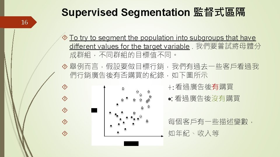
17 Supervised Segmentation監督式區隔 We might like to rank the variables by how good they are at predicting the value of the target. 我們想找出描述變數對目 標值預測能力的排名 In our example, what variable gives us the most information about the future churn rate of the population? Being a professional? Age? Place of residence? Income? Number of complaints to customer service? Amount of overage charges? 在我們預測顧客流失的案例，哪一個變數對顧客流 失率能給我們最多的資訊? 年紀嗎? 居住地嗎? 收入嗎? 跟客 服抱怨次數嗎? 超額費用金額嗎? 或是顧客是專業人士這個 變數嗎?

18 Supervised Segmentation監督式區隔 We now will look carefully into one useful way to select informative variables, and then later will show this technique can be used repeatedly to build a supervised segmentation. 接下來我們要介紹一個讓我們選取具傳遞訊 息能力變數的有用方法，之後我們會看如何用該方法去建立 監督督式區隔

19 Outline Models, Induction, and Prediction Supervised Segmentation Selecting Informative Attributes 選擇具傳遞訊息能力的屬性 Example: Attribute Selection with Information Gain Supervised Segmentation with Tree-Structured Models

20 Selecting Informative Attributes選擇具 傳遞訊息能力的屬性 The label over each head represents the value of the target variable (write-off or not). 每個人頭上的值代表目標值 (是否 有呆帳) Colors and shapes represent different predictor attributes. ( 顏色與形狀代表預測屬性值)

21 Selecting Informative Attributes選擇具 傳遞訊息能力的屬性 Attributes: head-shape: square, circular body-shape: rectangular, oval body-color: gray, white Target variable: write-off: Yes, No

22 Selecting Informative Attributes So let’s ask ourselves: which of the attributes would be best to segment these people into groups, in a way that will distinguish write-offs from non-writeoffs? 哪一個變數能將這些人分成有呆帳與沒有呆帳的兩組? Technically, we would like the resulting groups to be as pure as possible. By pure we mean homogeneous with respect to the target variable. If every member of a group has the same value for the target, then the group is pure. If there is at least one member of the group that has a different value for the target variable than the rest of the group, then the group is impure. 我們希望分開的兩組越純 越好。所謂純指的是在同一組內的人他們的目標值皆相同。

23 Selecting Informative Attributes Unfortunately, in real data we seldom expect to find a variable that will make the segments pure. 不幸的是當面 對真實資料時，我們很少能碰到一個變數能夠讓我們得到完 全純的分組

24 Selecting Informative Attributes Purity measure. 純度的度量 The most common splitting criterion is called information gain, and it is based on a purity measure called entropy. 最 常見的分組判斷標準叫做Information Gain, 它是基於一個純 度度量稱為entropy (熵 發音與低同) Both concepts were invented by one of the pioneers of information theory, Claude Shannon, in his seminal work in the field (Shannon, 1948). 兩個觀念都是資訊理論的先驅 Claude Shannon所提出

25 Selecting Informative Attributes Entropy is a measure of disorder(凌亂程度) that can be applied to a set, such as one of our individual segments. 熵 是呈現一組資料值的凌亂程度 Disorder corresponds to how mixed (impure) the segment is with respect to these properties of interest. 凌亂是指一組資 料值是如何的混雜、不純

26 Selecting Informative Attributes

27 Selecting Informative Attributes p(non-write-off) = 5/ 10 = 0. 5 p(write-off) = 5 / 10 = 0. 5 entropy(S) = - 0. 5 × log 2 (0. 5) – 0. 5 × log 2 (0. 5) = - 0. 5 × - 1 = 0. 5 + 0. 5 = 1 最不純

28 Selecting Informative Attributes p(non-write-off) = 10/ 10 = 1 p(write-off) = 0 / 10 = 0 entropy(S) = - 1 × log 2 (1) – 0 × log 2 (0) = -1 × 0 - 0 × - = 0 + 0 = 0 最純

29 Selecting Informative Attributes p(non-write-off) = 7 / 10 = 0. 7 p(write-off) = 3 / 10 = 0. 3 entropy(S) = - 0. 7 × log 2 (0. 7) – 0. 3 × log 2 (0. 3) ≈ - 0. 7 × - 0. 51 - 0. 3 × - 1. 74 ≈ 0. 88

30 Selecting Informative Attributes

31 Selecting Informative Attributes entropy(parent) = - p( • ) × log 2 p( • ) - p( ☆ ) × log 2 p( ☆ ) ≈ - 0. 53 × - 0. 9 - 0. 47 × - 1. 1 ≈ 0. 99 (very impure)

32 Selecting Informative Attributes The entropy of the left child is: entropy(Balance < 50 K) = - p( • ) × log 2 p( • ) - p( ☆ ) × log 2 p( ☆ ) ≈ - 0. 92 × ( - 0. 12) - 0. 08 × ( - 3. 7) ≈ 0. 39 The entropy of the right child is: entropy(Balance ≥ 50 K) = - p( • ) × log 2 p( • ) - p( ☆ ) × log 2 p( ☆ ) ≈ - 0. 24 × ( - 2. 1) - 0. 76 × ( - 0. 39) ≈ 0. 79

33 Selecting Informative Attributes Information Gain = entropy(parent) - (p(Balance < 50 K) × entropy(Balance < 50 K) + p(Balance ≥ 50 K) × entropy(Balance ≥ 50 K)) ≈ 0. 99 – (0. 43 × 0. 39 + 0. 57 × 0. 79) ≈ 0. 37

34 Selecting Informative Attributes entropy(parent) ≈ 0. 99 entropy(Residence=OWN) ≈ 0. 54 entropy(Residence=RENT) ≈ 0. 97 entropy(Residence=OTHER) ≈ 0. 98 Information Gain ≈ 0. 13

35 Numeric variables We have not discussed what exactly to do if the attribute is numeric. Numeric variables can be “discretized” (離散化、區段化)by choosing a split point(or many split points). For example, Income could be divided into two or more ranges. Information gain can be applied to evaluate the segmentation created by this discretization of the numeric attribute. We still are left with the question of how to choose the split point(s) for the numeric attribute. Conceptually, we can try all reasonable split points, and choose the one that gives the highest information gain.

36 Outline Models, Induction, and Prediction Supervised Segmentation Selecting Informative Attributes Example: Attribute Selection with Information Gain 用 Information Gain去選取屬性 Supervised Segmentation with Tree-Structured Models

37 Example: Attribute Selection with Information Gain用Information Gain去選 取屬性 For a dataset with instances described by attributes and a target variable. 當我們拿到一個多筆資料的資料集，每筆資料都由一些 屬性所描繪，同時有一個目標變數 We can determine which attribute is the most informative with respect to estimating the value of the target variable. 我們首先決 定哪個屬性對於估計目標變數值是最具傳遞訊息能力 We also can rank a set of attributes by their informativeness, in particular by their information gain. 我們計算每個變數的 information gain，然後根據information gain的值將變數排序，從 大到小

38 Example: Attribute Selection with Information Gain 用Information Gain去選 取屬性 This is a classification problem because we have a target variable, called edible? , with two values yes (edible) and no (poisonous), specifying our two classes. 下面的例子是一個 分類問題，有一個目標變數叫做可吃嗎? 它有兩個可能值， 亦即YES(可吃)與NO(有毒) Each of the rows in the training set has a value for this target variable. We will use information gain to answer the question: “Which single attribute is the most useful for distinguishing edible (edible? =Yes) mushrooms from poisonous (edible? =No) ones? ” 在訓練資料裡，每一列的資 料，都有其目標值。我們要用information gain去回答: 哪一 個屬性最能分辨可吃與有毒的香菇?

香菇資料集 39 香菇帽 香菇柄 GILL: 香菇的菌褶 We use 5, 644 examples from the dataset, 香菇面紗 comprising 2, 156 poisonous(有毒) and 3, 488 edible(可吃) mushrooms 23 attributes UCI dataset SPORE: 香菇孢子

40 Example: Attribute Selection with Information Gain 用Information Gain去選 取屬性 Figure 3 -6. Entropy chart for the entire Mushroom dataset (香菇資料集 Entropy圖). The entropy for the entire dataset is 0. 96, so 96% of the area is shaded. entropy(parent) ≈ 0. 96

41 Example: Attribute Selection with Information Gain 用Information Gain去選 取屬性 Figure 3 -6. This is our starting entropy—any informative attribute should produce a new graph with less shaded area. ( 這是我們的起點， 任何具傳遞訊息的 屬性應該讓陰影區 變小)

42 Example: Attribute Selection with Information Gain 用Information Gain去選 取屬性 Figure 3 -7. Entropy chart for the Mushroom dataset as split by GILLCOLOR (菌褶顏 色) whose values are coded as y(yellow), u (purple), n (brown), and so on.

43 Example: Attribute Selection with Information Gain 用Information Gain去選 取屬性 Figure 3 -7. The width of each attribute represents what proportion of the dataset has that value, and the height is its entropy. (每個區塊代 表一個屬性值，其寬度 代表佔全體比例，寬度 代表entropy)

44 Example: Attribute Selection with Information Gain 用Information Gain去選 取屬性 Figure 3 -7. 因此如 果選用GILLCOLOR做為分類 的變數， Information Gain就 是: Fig 3 -6的陰影 區 – Fig 3 -7的陰影 區，陰影區減少愈 多愈好。

45 Example: Attribute Selection with Information Gain 用Information Gain去選 取屬性 Figure 3 -8. Entropy chart for the Mushroom dataset as split by SPORE-PRINT -COLOR (孢子纹顏色). A few of the values, such as h (chocolate), specify the target value perfectly and thus produce zeroentropy bars. But notice that they don’t account for very much of the population, only about 30%. (有些屬性值讓 entropy=0)

46 Example: Attribute Selection with Information Gain 用Information Gain去選 取屬性 Figure 3 -9. Entropy chart for the Mushroom dataset as split by ODOR ( 氣味).

47 Example: Attribute Selection with Information Gain 用Information Gain去選 取屬性 In fact, ODOR has the highest information gain of any attribute in the Mushroom dataset. It can reduce the dataset’s total entropy to about 0. 1, which gives it an information gain of 0. 96 – 0. 1 = 0. 86. Many odors are completely characteristic of poisonous or edible mushrooms, so odor is a very informative attribute to check when considering mushroom edibility. See footnote 5 on page 61.

48 Example: Attribute Selection with Information Gain 用Information Gain去選 取屬性 If you’re going to build a model to determine the mushroom edibility using only a single feature, you should choose its odor. 如果你只用一個屬性去決定香菇是否可吃，你應該用 它的味道 If you were going to build a more complex model you might start with the attribute ODOR before considering adding others. 如果你要建立一個較複雜的模型，你可以從味道開始 區隔香菇，之後再用別的屬性 In fact, this is exactly the topic of the next section.

49 Outline Models, Induction, and Prediction Supervised Segmentation Selecting Informative Attributes Example: Attribute Selection with Information Gain Supervised Segmentation with Tree-Structured Models 用樹狀 模型進行監督式區隔

50 Supervised Segmentation with Tree. Structured Models 用樹狀模型進行監督 式區隔 Let’s continue on the topic of creating a supervised segmentation, because as important as it is, attribute selection alone does not seem to be sufficient. 我們繼續討論建立監督式區隔這個議題 If we select the single variable that gives the most information gain, we create a very simple segmentation. 當我們用一個變數去 區隔資料集的成員時，我們得到一個簡單的區隔 If we select multiple attributes each giving some information gain, it’s not clear how to put them together. 如果要用多個變數，要如何 進行區隔呢?

51 Supervised Segmentation with Tree. Structured Models 用樹狀模型進行監督 式區隔 We now introduce an elegant application of the ideas we’ve developed for selecting important attributes, to produce a multivariate (multiple attribute) supervised segmentation. 下面我們 介紹一個很優雅的方法，讓我們建立一個多變數監督式區隔

52 Supervised Segmentation with Tree. Structured Models用樹狀模型進行監督式 區隔 Consider a segmentation of the data to take the form of a “tree, ” such as that shown in Figure 3 -10.

53 Supervised Segmentation with Tree. Structured Models The values of Claudio’s attributes are Balance=115 K, Employed=No, and Age=40.

54 Supervised Segmentation with Tree. Structured Models 用樹狀模型進行監督式 區隔 There are many techniques to induce a supervised segmentation from a dataset. One of the most popular is to create a tree-structured model (tree induction). 有許多方法 可以從一個資料集去歸納出監督式區隔，用樹狀模型進行歸 納是最常見的方式之一 These techniques are popular because tree models are easy to understand, and because the induction procedures are elegant (simple to describe) and easy to use. They are robust to many common data problems and are relatively efficient. 因為樹狀模型容易了解，建立過程容易說明，模型 也容易使用。

55 Supervised Segmentation with Tree. Structured Models 用樹狀模型進行監督式 區隔 Combining the ideas introduced above, the goal of the tree is to provide a supervised segmentation— more specifically, to partition the instances, based on their attributes, into subgroups that have similar values for their target variables. 樹狀模型的目標當然是為了監督式區隔---根 據屬性將資料分組，使得同組資料的目標變數值盡量相同 We would like for each “leaf ” segment to contain instances that tend to belong to the same class. 我們希望每一個葉分 組內的資料能屬於同一類別

56 Supervised Segmentation with Tree. Structured Models 用樹狀模型進行監督式 區隔 To illustrate the process of classification tree induction, consider the very simple example set shown previously in Figure 3 -2 為了解釋分類樹歸納的過程，我們用之前見過的 案例

57 Selecting Informative Attributes 選取具 傳遞訊息能力的屬性 Attributes: head-shape: square, circular body-shape: rectangular, oval body-color: gray, white Target variable: write-off: Yes, No

58 Supervised Segmentation with Tree. Structured Models 用樹狀模型進行監督式 區隔 Figure 3 -11. First partitioning: splitting on body shape (rectangular versus oval). 先用身體形狀(長 方形與橢圓形)將資料 分組

59 Supervised Segmentation with Tree. Structured Models 用樹狀模型進行監督式 區隔 Figure 3 -12. Second partitioning: the oval body people subgrouped by head type.

60 Supervised Segmentation with Tree. Structured Models 用樹狀模型進行監督式 區隔 Figure 3 -13. Third partitioning: the rectangular body people subgrouped by body color.

61 Figure 3 -14. The classification tree resulting from the splits done in Figure 311 to Figure 3 -13.

62 Supervised Segmentation with Tree. Structured Models 用樹狀模型進行監督式 區隔 In summary, the procedure of classification tree induction is a recursive process of divide and conquer, where the goal at each step is to select an attribute to partition the current group into subgroups that are as pure as possible with respect to the target variable. 總的來說，分類樹歸納的過程 是一個各個擊破的重覆過程，是在每一步選一個屬性，將當 下的群組區隔成子群組，目的是讓每一子群組的成員其目標 值越相同越好

63 Supervised Segmentation with Tree. Structured Models 用樹狀模型進行監督式 區隔 When are we done? (In other words, when do we stop recursing? ) 但此區隔 作何時完成呢? It should be clear that we would stop when the nodes are pure, or when we run out of variables to split on. 當每個子群組內成員的目標 值都一樣的時候，當然就無須再區隔 But we may want to stop earlier; we will return to this question in Chapter 5. 有時候我們可能選擇提早停止區隔，課本第五章會討論這 個議題

64 Visualizing Segmentations 用視覺化方式 呈現區隔 It is instructive to visualize exactly how a classification tree partitions the instance space. 用視覺化方式去看某個分類如 何將樣本空間分隔常對了解問題常會有幫助 The instance space is simply the space described by the data features. 樣本空間是由資料的屬性來描述 A common form of instance space visualization is a scatterplot (散佈圖) on some pair of features, used to compare one variable against another to detect correlations and relationships. 一個常被使用來觀察樣本空間的 具是用 兩個屬性繪製的2 D散佈圖，它可以幫我們找出針對目標值兩 個屬性間的關聯性

65 Visualizing Segmentations Though data may contain dozens or hundreds of variables, it is only really possible to visualize segmentations in two or three dimensions at once 雖然 資料可能有數十甚至數百個變數，但同時間只有用 2 D或 3 D 方式才容易用視覺化看樣本區隔 Visualizing models in instance space in a few dimensions is useful for understanding the different types of models because it provides insights that apply to higher dimensional spaces as well 我們用視覺化方式在少數維度 下看模型能幫助我們了解不同種類的模型的本質與表現

66 Visualizing Segmentations *The black dots correspond to instances of the class Write-off. *The plus signs correspond to instances of class non-Write-off.

67 Trees as Sets of Rules You classify a new unseen instance by starting at the root node and following the attribute tests downward until you reach a leaf node, which specifies the instance’s predicted class. If we trace down a single path from the root node to a leaf, collecting the conditions as we go, we generate a rule. Each rule consists of the attribute tests along the path connected with AND.

68 Trees as Sets of Rules

69 Trees as Sets of Rules IF (Balance < 50 K) AND (Age < 50) THEN Class=Write-off IF (Balance < 50 K) AND (Age ≥ 50) THEN Class=No Write-off IF (Balance ≥ 50 K) AND (Age < 45) THEN Class=No Write-off

70 Trees as Sets of Rules The classification tree is equivalent to this rule set. 分類 樹與規則集相等 Every classification tree can be expressed as a set of rules this way. 每一棵分類樹都可以用這種方法表示成一組 規則

71 Probability Estimation In many decision-making problems, we would like a more informative prediction than just a classification. 對許多決策 問題而言，我們想要的是一個較分類更能傳遞訊息的預測 For example, in our churn prediction problem. If we have the customers’ probability of leaving when their contracts are about to expire, we could rank them and use a limited incentive budget to the highest probability instances. 例如 對流失預測而言，我們想要將顧客按流失機率排序，然後將 有限的行銷預算花在較高機率的顧客身上

72 Probability Estimation Alternatively, we may want to allocate our incentive budget to the instances with the highest expected loss, for which you’ll need the probability of churn. 或者我們想將預算花 在期望損失高的顧客身上，為此你必須能算出顧客流失機率

73 Probability Estimation Tree

74 Probability Estimation If we are satisfied to assign the same class probability to every member of the segment corresponding to a tree leaf, we can use instance counts at each leaf to compute a class probability estimate. 如果我們將相同的機率值給葉節點內的 每個成員，那我們可以用每個葉節點內的個體數去估計類別 的機率 For example, if a leaf contains n positive instances and m negative instances, the probability of any new instance being positive may be estimated as n/(n+m). This is called a frequency-based estimate of class membership probability. 如果+ve案例有n個，-ve案例有m個，則新案例 是+ve的機率為n/(n+m).

75 Probability Estimation A problem: we may be overly optimistic about the probability of class membership for segments with very small numbers of instances. At the extreme, if a leaf happens to have only a single instance, should we be willing to say that there is a 100% probability that members of that segment will have the class that this one instance happens to have? This phenomenon is one example of a fundamental issue in data science (“overfitting”).

76 Probability Estimation Instead of simply computing the frequency, we would often use a “smoothed” version of the frequency-based estimate, known as the Laplace correction, the purpose of which is to moderate the influence of leaves with only a few instances. The equation for binary class probability estimation becomes:

77 Example: Addressing the Churn Problem with Tree Induction We have a historical data set of 20, 000 customers. At the point of collecting the data, each customer either had stayed with the company or had left (churned).

78 Example: Addressing the Churn Problem with Tree Induction 用樹狀歸納法處理預測 客戶流失問題

79 Example: Addressing the Churn Problem with Tree Induction How good are each of these variables individually? 單一變數 有多好 (預測客戶流失上) For this we measure the information gain of each attribute, as discussed earlier. Specifically, we apply Equation 3 -2 to each variable independently over the entire set of instances, to see what each gains us. 為此，我們計算 每一變數的information gain.

80

81

82 Example: Addressing the Churn Problem with Tree Induction The answer is that the table ranks each feature by how good it is independently, evaluated separately on the entire population of instances. Nodes in a classification tree depend on the instances above them in the tree. 在分類樹內的一個節點內是用哪些 變數，端賴在該節點剩下哪些資料需要被區隔

83 Example: Addressing the Churn Problem with Tree Induction Therefore, except for the root node, features in a classification tree are not evaluated on the entire set of instances. 因此，除了在根節點以外，在其他節點並不是用 全部的資料計算information gain The information gain of a feature depends on the set of instances against which it is evaluated, so the ranking of features for some internal node may not be the same as the global ranking. 一個變數的information gain是多少跟 是哪些資料用來計算IG有關，所以在決策樹內的節點計算變 數的排序，跟在根節點計算變數的排序未必相同