1 Categorical Data Analysis HYPOTHESIS TESTING Data Types

1 Categorical Data Analysis HYPOTHESIS TESTING

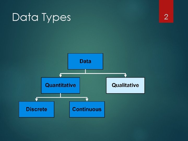
Data Types 2

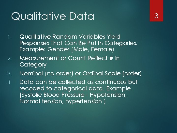
Qualitative Data 1. 2. 3. 4. Qualitative Random Variables Yield Responses That Can Be Put In Categories. Example: Gender (Male, Female) Measurement or Count Reflect # in Category Nominal (no order) or Ordinal Scale (order) Data can be collected as continuous but recoded to categorical data. Example (Systolic Blood Pressure - Hypotension, Normal tension, hypertension ) 3

4 2 Test of Independence Between 2 Categorical Variables

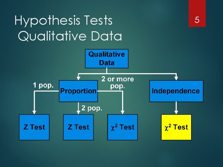
Hypothesis Tests Qualitative Data 5

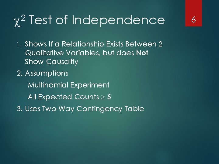
2 1. Test of Independence Shows If a Relationship Exists Between 2 Qualitative Variables, but does Not Show Causality 2. Assumptions Multinomial Experiment All Expected Counts 5 3. Uses Two-Way Contingency Table 6

2 Test of Independence Contingency Table 7 Shows # Observations From 1 Sample Jointly in 2 Qualitative Variables 1.

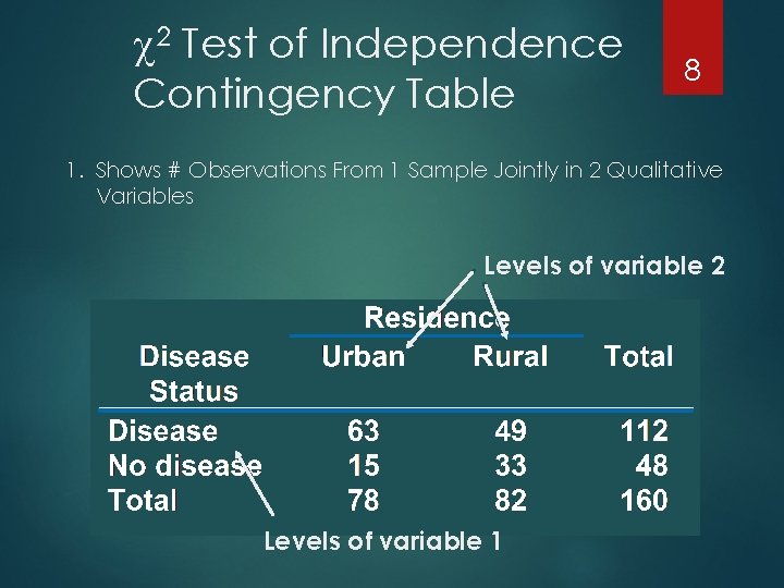
2 Test of Independence Contingency Table 8 1. Shows # Observations From 1 Sample Jointly in 2 Qualitative Variables Levels of variable 2 Levels of variable 1

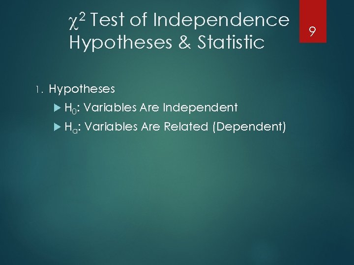
2 Test of Independence Hypotheses & Statistic 1. Hypotheses H 0: Variables Are Independent H a: Variables Are Related (Dependent) 9

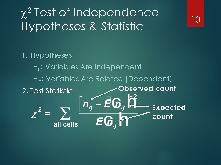
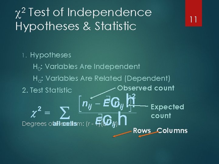
2 Test of Independence Hypotheses & Statistic 1. Hypotheses H 0: Variables Are Independent Ha: Variables Are Related (Dependent) Observed count 2. Test Statistic Expected count 10

2 Test of Independence Hypotheses & Statistic 1. Hypotheses H 0: Variables Are Independent Ha: Variables Are Related (Dependent) Observed count 2. Test Statistic Degrees of Freedom: (r - 1)(c - 1) Expected count Rows Columns 11

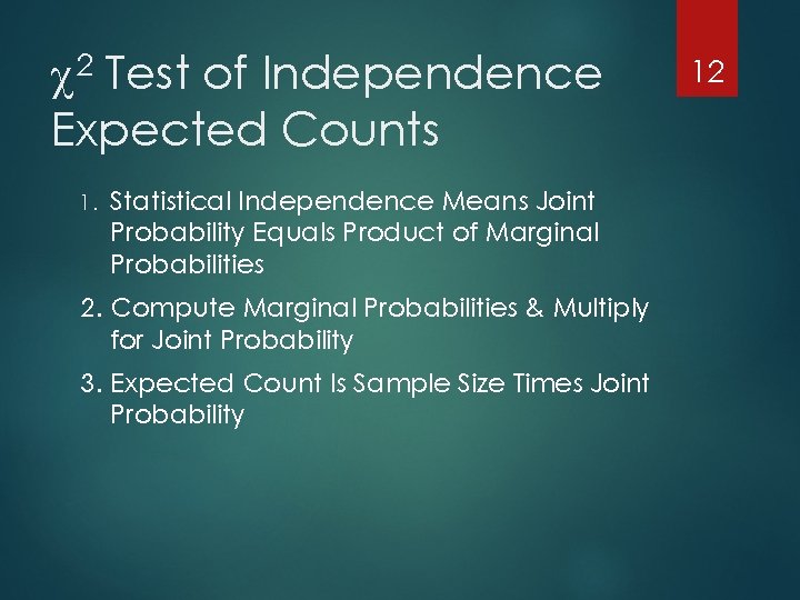
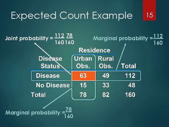
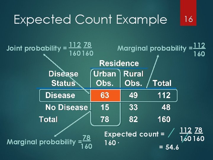
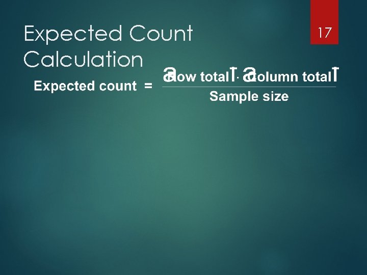
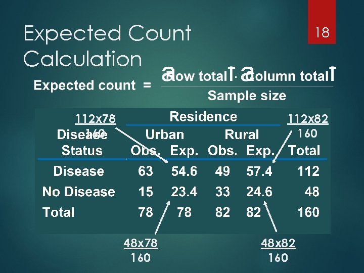
2 Test of Independence Expected Counts 1. Statistical Independence Means Joint Probability Equals Product of Marginal Probabilities 2. Compute Marginal Probabilities & Multiply for Joint Probability 3. Expected Count Is Sample Size Times Joint Probability 12

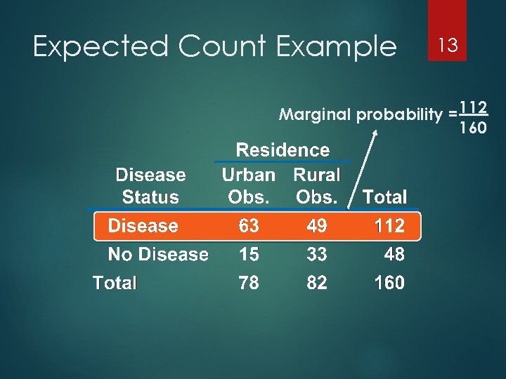
Expected Count Example 13 Marginal probability = 112 160

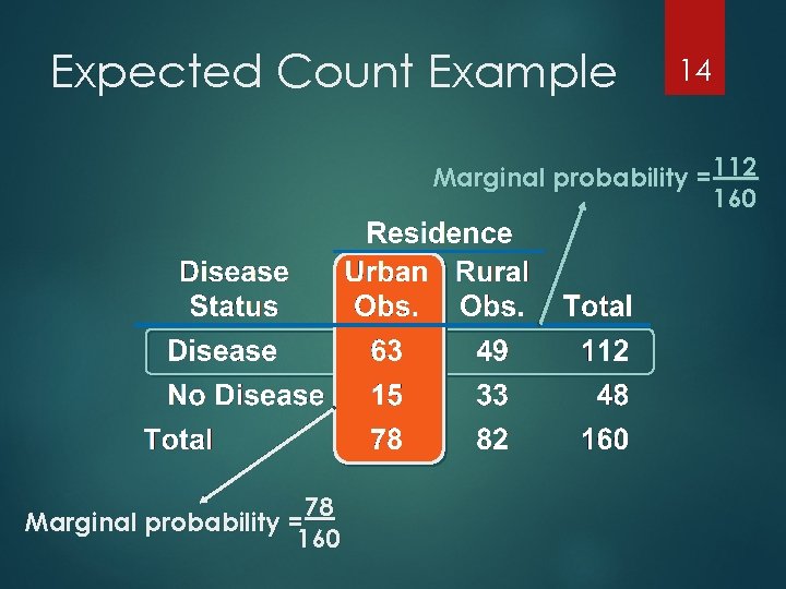
Expected Count Example 14 Marginal probability = 112 160 78 Marginal probability = 160

Expected Count Example 112 78 Joint probability = 160 78 Marginal probability = 160 15 Marginal probability = 112 160

Expected Count Example 112 78 Joint probability = 160 78 Marginal probability = 160 16 Marginal probability = 112 160 Expected count = 160· = 54. 6 112 78 160

Expected Count Calculation 17

Expected Count Calculation 112 x 78 160 18 112 x 82 160 48 x 78 160 48 x 82 160

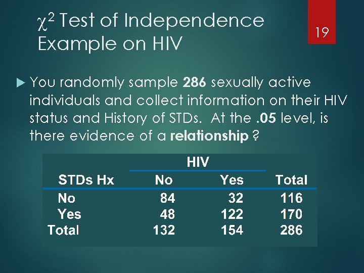
2 Test of Independence Example on HIV 19 You randomly sample 286 sexually active individuals and collect information on their HIV status and History of STDs. At the. 05 level, is there evidence of a relationship ?

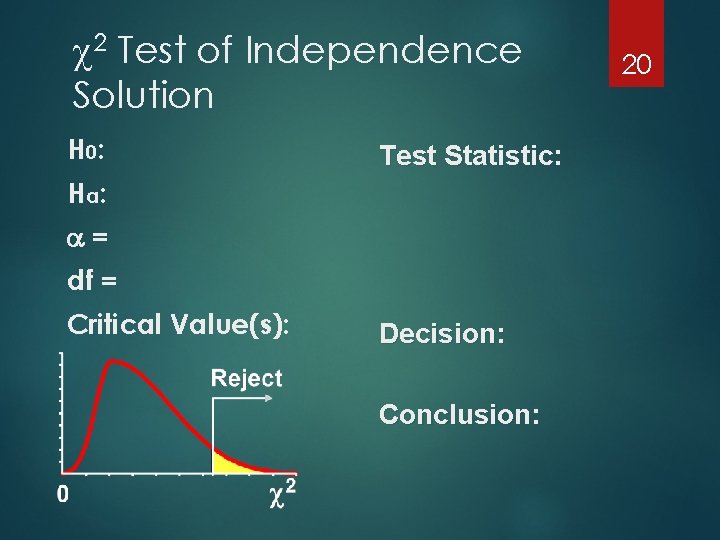
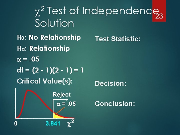
2 Test of Independence Solution H 0: Test Statistic: Ha : = df = Critical Value(s): Decision: Conclusion: 20

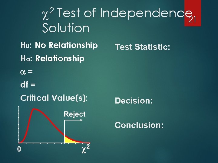
2 Test of Independence 21 Solution H 0: No Relationship Test Statistic: Ha : Relationship = df = Critical Value(s): Decision: Conclusion:

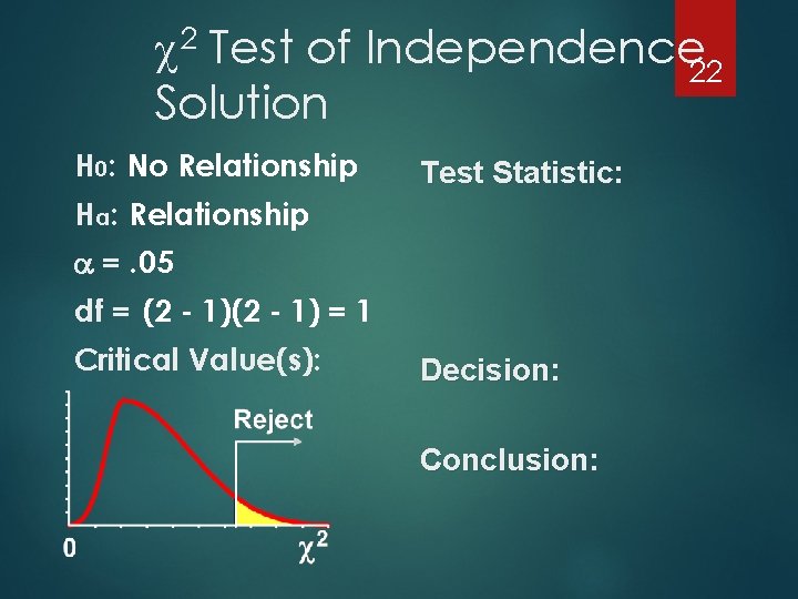
2 Test of Independence 22 Solution H 0: No Relationship Test Statistic: Ha : Relationship =. 05 df = (2 - 1) = 1 Critical Value(s): Decision: Conclusion:

2 Test of Independence 23 Solution H 0: No Relationship Test Statistic: Ha : Relationship =. 05 df = (2 - 1) = 1 Critical Value(s): =. 05 Decision: Conclusion:

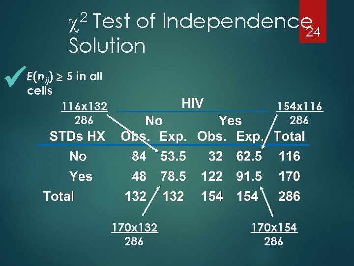
2 Test of Independence 24 Solution E (nij) 5 in all cells 116 x 132 286 154 x 116 286 170 x 132 286 170 x 154 286

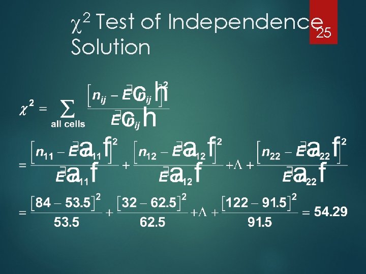
2 Test of Independence 25 Solution

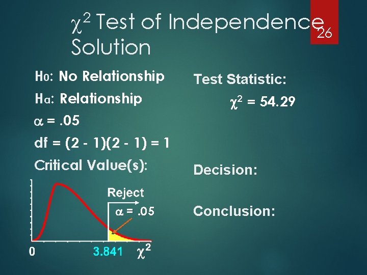
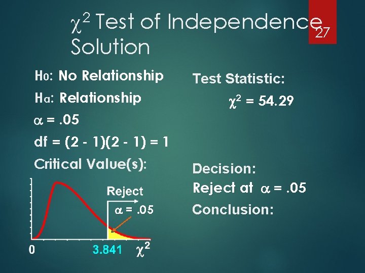
2 Test of Independence 26 Solution H 0: No Relationship Ha : Relationship Test Statistic: 2 = 54. 29 =. 05 df = (2 - 1) = 1 Critical Value(s): =. 05 Decision: Conclusion:

2 Test of Independence 27 Solution H 0: No Relationship Ha : Relationship Test Statistic: 2 = 54. 29 =. 05 df = (2 - 1) = 1 Critical Value(s): =. 05 Decision: Reject at =. 05 Conclusion:

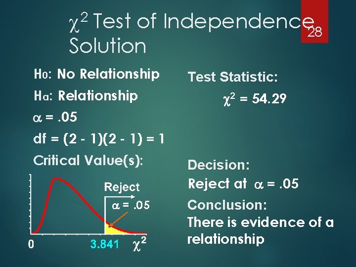
2 Test of Independence 28 Solution H 0: No Relationship Ha : Relationship Test Statistic: 2 = 54. 29 =. 05 df = (2 - 1) = 1 Critical Value(s): =. 05 Decision: Reject at =. 05 Conclusion: There is evidence of a relationship

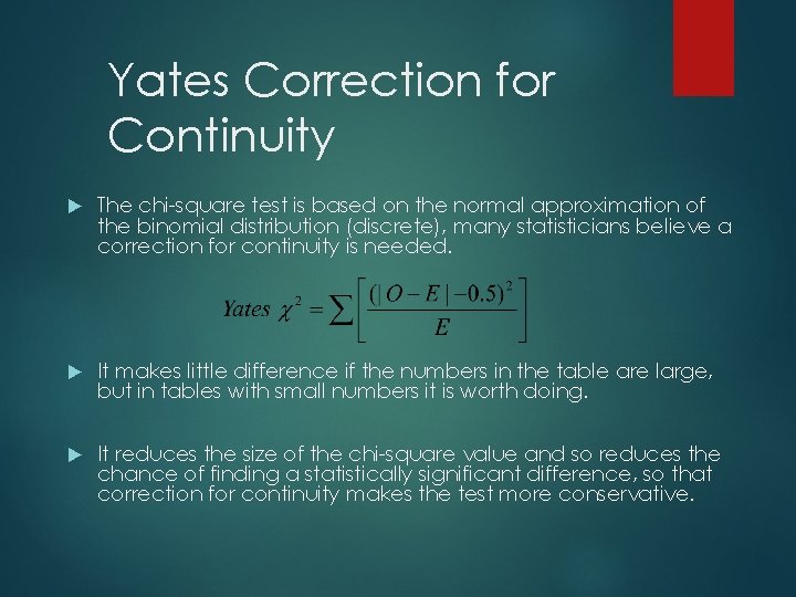
Yates Correction for Continuity The chi-square test is based on the normal approximation of the binomial distribution (discrete), many statisticians believe a correction for continuity is needed. It makes little difference if the numbers in the table are large, but in tables with small numbers it is worth doing. It reduces the size of the chi-square value and so reduces the chance of finding a statistically significant difference, so that correction for continuity makes the test more conservative.

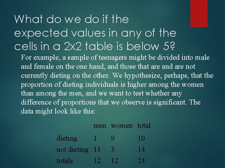
What do we do if the expected values in any of the cells in a 2 x 2 table is below 5? For example, a sample of teenagers might be divided into male and female on the one hand, and those that are and are not currently dieting on the other. We hypothesize, perhaps, that the proportion of dieting individuals is higher among the women than among the men, and we want to test whether any difference of proportions that we observe is significant. The data might look like this: men women total dieting 1 not dieting 11 totals 12 9 3 12 10 14 24

The question we ask about these data is: knowing that 10 of these 24 teenagers are dieters, what is the probability that these 10 dieters would be so unevenly distributed between the girls and the boys? If we were to choose 10 of the teenagers at random, what is the probability that 9 of them would be among the 12 girls, and only 1 from among the 12 boys? --Hypergeometric distribution! --Fisher’s exact test uses hypergeometric distribution to calculate the “exact” probability of obtaining such set of the values.