1 AP STATISTICS LESSON 11 1 DAY 1

1. AP STATISTICS LESSON 11 – 1 (DAY 1) INFERENCE FOR THE MEAN OF A POPULATION

ESSENTIAL QUESTION: What are the procedures for making inferences when the populations standard deviation is unknown? Objectives: l To become familiar with the procedures for inference when the populations standard deviation is unknown. l To use t calculations and procedures that will lead to making inferences.

Introduction This chapter describes confidence intervals and significance tests for the mean of a single population and for comparing the means of two populations.

Inference for the Mean of a Population Confidence intervals and tests of significance for the mean μ of a normal population are based on the sample mean x. The sampling distribution of x has μ as its mean. That is an unbiased estimator of the unknown μ. l In the previous chapter we make the unrealistic assumption that we knew the value of σ. In practice, σ is unknown. l

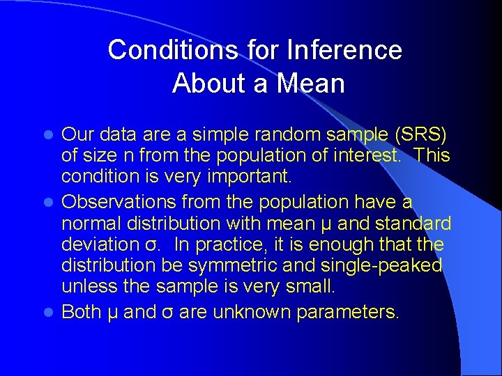
Conditions for Inference About a Mean Our data are a simple random sample (SRS) of size n from the population of interest. This condition is very important. l Observations from the population have a normal distribution with mean μ and standard deviation σ. In practice, it is enough that the distribution be symmetric and single-peaked unless the sample is very small. l Both μ and σ are unknown parameters. l

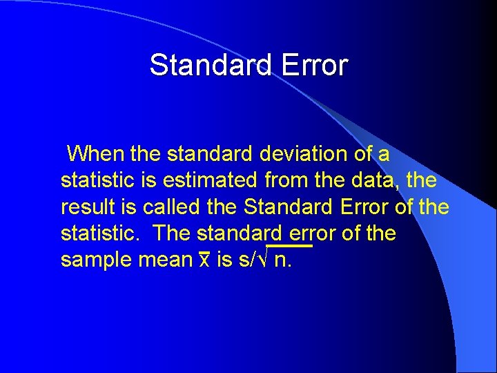
Standard Error When the standard deviation of a statistic is estimated from the data, the result is called the Standard Error of the statistic. The standard error of the sample mean x is s/√ n.

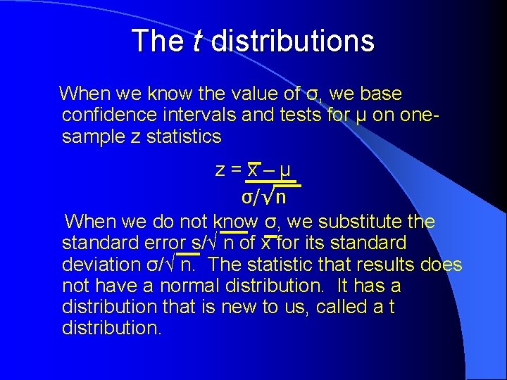
The t distributions When we know the value of σ, we base confidence intervals and tests for μ on onesample z statistics z=x–μ σ/√n When we do not know σ, we substitute the standard error s/√ n of x for its standard deviation σ/√ n. The statistic that results does not have a normal distribution. It has a distribution that is new to us, called a t distribution.

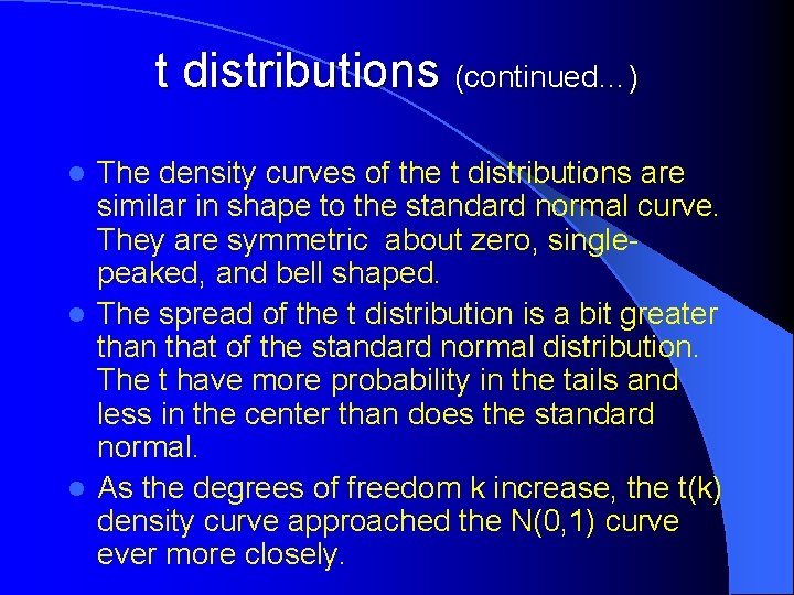
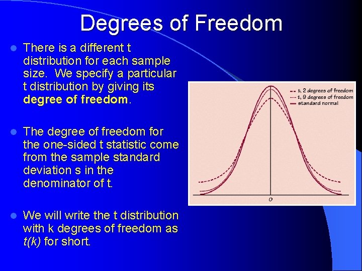
t distributions (continued…) The density curves of the t distributions are similar in shape to the standard normal curve. They are symmetric about zero, singlepeaked, and bell shaped. l The spread of the t distribution is a bit greater than that of the standard normal distribution. The t have more probability in the tails and less in the center than does the standard normal. l As the degrees of freedom k increase, the t(k) density curve approached the N(0, 1) curve ever more closely. l

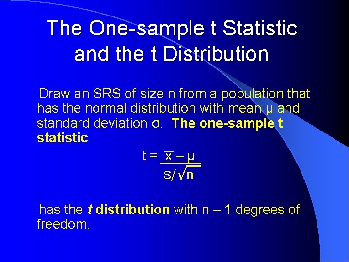
The One-sample t Statistic and the t Distribution Draw an SRS of size n from a population that has the normal distribution with mean μ and standard deviation σ. The one-sample t statistic t= x–μ S/√n has the t distribution with n – 1 degrees of freedom.

Degrees of Freedom l There is a different t distribution for each sample size. We specify a particular t distribution by giving its degree of freedom. l The degree of freedom for the one-sided t statistic come from the sample standard deviation s in the denominator of t. l We will write the t distribution with k degrees of freedom as t(k) for short.

Example 11. 1 Page 619 Using the “t Table” What critical value t* from Table C (back cover of text book, often referred to as the “t table”) would you use for a t distribution with 18 degrees of freedom having probability 0. 90 to the left of t?

More Practice… What critical value t* from Table C should be used for a confidence interval for the mean of the population in each of the following situations? 1. A 90% confidence interval based on n = 12 observations? 2. A 95% confidence interval froman SRS of 30 observations 3. An 80% confidence interval from a sample of size 18