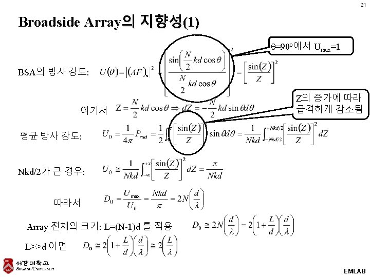
1 Antenna beam synthesis EMLAB 2 EMLAB 5

1 Antenna beam synthesis EMLAB

2 EMLAB
 배열 소자가 이산적(Discrete)으로 분포하기 때문에 각 단 위")
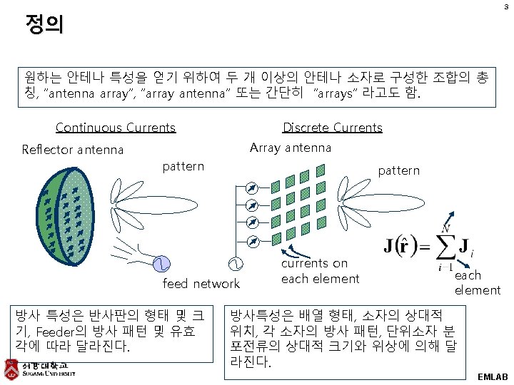
5 Complex Excitation Coefficients(복소 급전 계수) 배열 소자가 이산적(Discrete)으로 분포하기 때문에 각 단 위 “소자의 크기와 위상”을 독립적으로 제어할 수 있다. “excitation coefficients”(복소 급전 계수) phase shifters amplifiers (or attenuators) element #1 This is called Beam forming network or Feed network Array elements element #n EMLAB
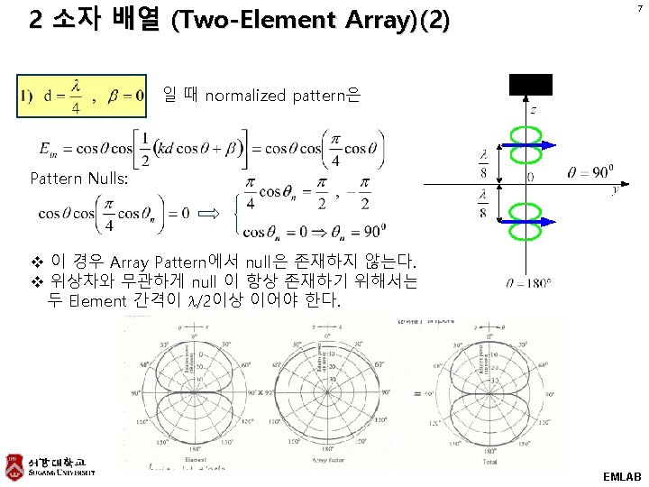
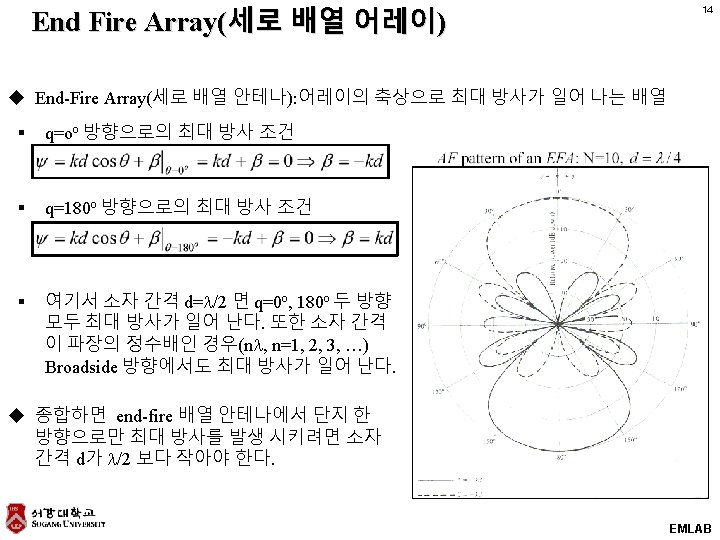
 8 일때 Pattern Nulls: : 2)의 결과와 q= 90")
예: 2소자 배열의 Array Factor(3) 8 일때 Pattern Nulls: : 2)의 결과와 q= 90 o에 대해 대칭 EMLAB
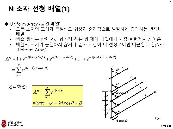
 § AF의 Nulls : maximum § AF의 Maximum m=0는")
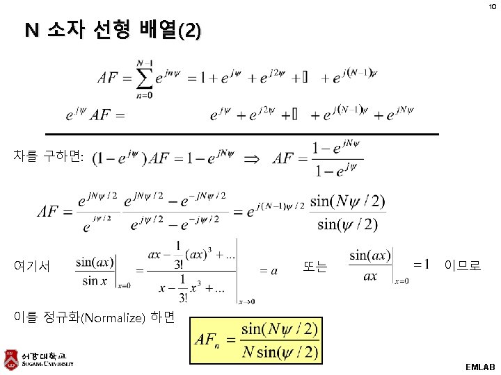
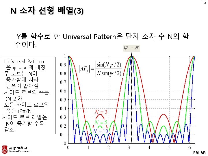
11 N 소자 선형 배열(3) § AF의 Nulls : maximum § AF의 Maximum m=0는 main lobe에 해당하며 이 때 § main lobe의 HPBW § secondary maxima: minor lobe의 maxima EMLAB
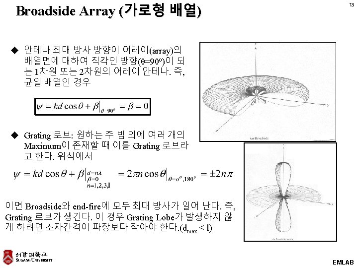
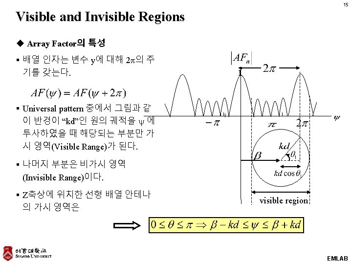

16 Grating Lobes Phenomenon § 반경 kd인 원을 y에 투사했을 때 Universal Pattern상에 있는 하나 이상의 Peak가 이 범위에 속하면 Grating Lobe 현상이 발생한다. 1 § 즉, 주 빔과 동일한 크기를 갖는 다른 Lobe가 존재하게 된다. § Grating Lobe를 피하기 위해 일반 적으로 다음 조건을 만족해야 한 다. grating lobes major lobe They have the same strength ! visible region Example : , no grating lobe occurs EMLAB

18 Ordinary Endfire Array 보통 end-fire 조건은 Normalized Array Factor가 q = 0 o 또는 180 o 에서 최대가 되도 록 해야 한다. end-fire beam Case II: 여기서 이때 end-fire Array가 0 o 또는 180 o 에서 dominant한 주 빔을 갖도록 하기 위해서는 적어도 p/N 만 큼은 Visible Range를 감소시킬 필요가 있다. Case I: 또는 EMLAB
 universal pattern End-fire beam z N=5 원의 반경 Very")
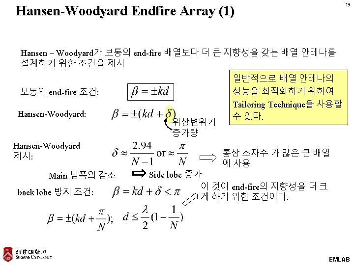
20 Hansen-Woodyard Endfire Array (2) universal pattern End-fire beam z N=5 원의 반경 Very low back lobes § H. W. 배열은 보통의 배열에 비해 지향성이 2. 5 d. B 증가하는 대신 side lobe가 4 d. B 정도 증가 EMLAB
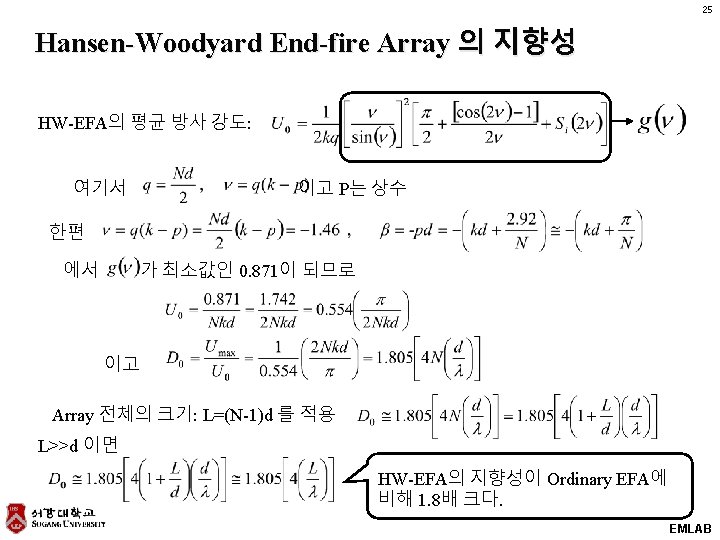
에서 반 전력 빔폭이 2")
Array의 설계 26 u 배열 축으로부터 30 o (q=30 o)에서 반 전력 빔폭이 2 o인 uniform linear scanning array를 설계 단, 소자 간격 은 l/4 § Excitation: Amplitude: Uniform Progressive Phase: § Array Length: 49. 75 l § Element Number: § Directivity: 100. 72(20. 03 d. B) EMLAB

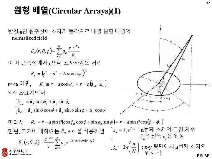
N-Element Linear Array: 3 D 특성 27 § Array축이 임의의 방향으로 배열된 경우 Array축과 관측점까지의 Radius Vector가 이루는 각 Excitation Amplitude § Array 축이 z 방향인 경우 Progressive Phase Excitation 지금까지의 결과와 동일 § Array 축이 x 방향이면 § Array 축이 y 방향이면 EMLAB
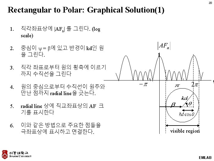
 Example : 4 -element linear array x Uniform")
29 Rectangular to Polar: Graphical Solution(2) Example : 4 -element linear array x Uniform array configuration : progressive phase shift Excitation … d z …… Note: Steps : 1. 2. 중심이 “p/2”에 있고 반경이 “p”인 원을 그린다. 3. 수직선을 긋는다. 4. 수직선이 원주와 만난 점까지 radial line을 긋는다. 5. radial line 상에 직교좌표상의 AF 크기를 표시한다 EMLAB
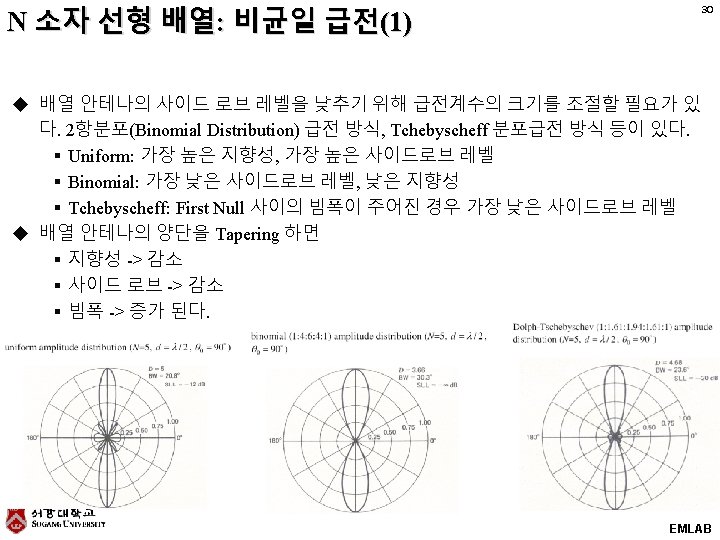
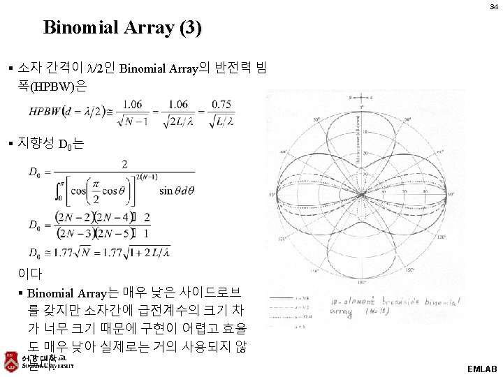
 § 2항 계수(Binomial Coefficients)를 갖는 선형 배열 안테나는 소자간 간격이")
32 Binomial Array (1) § 2항 계수(Binomial Coefficients)를 갖는 선형 배열 안테나는 소자간 간격이 반파장 이하이면 사이드로브를 발생시키지 않는다. 실수 여기서 이 것은 Z에 대한 (N-1) 차 다항식 소자수가 2개일 때: No sidelobes! For broadside 1 1 Observe: 1 1 1 2 (Z+1)=1+2 Z+Z 2 = X 1 Element pattern Array factor Overall pattern EMLAB
 1 4 -element binomial : AF=(1+Z)3=1+3 Z+3 Z 2+Z 3")
33 Binomial Array (2) 1 4 -element binomial : AF=(1+Z)3=1+3 Z+3 Z 2+Z 3 1 5 -element binomial : AF=(1+Z)4=1+4 Z+6 Z 2+4 Z 3+Z 4 N-element binomial : AF=(1+Z)N-1 Pascal’s triangle to create binomial coefficients : 2 1 1 2 3 1 4 1 3 6 1 4 1 N 1 2 3 4 5. . . 1 1 2 1 1 3 3 1 1 4 6 4 1 ……………… EMLAB
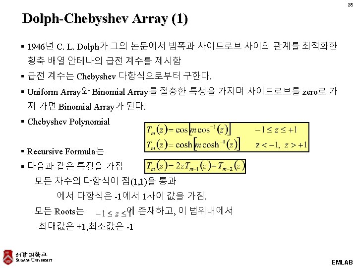
 The first four Chebyshev polynomials Tn(x). EMLAB")
36 Figure 5. 16 (p. 251) The first four Chebyshev polynomials Tn(x). EMLAB
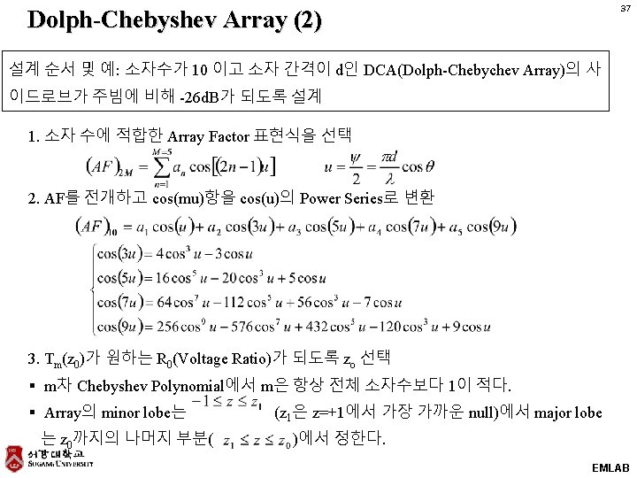
 3. 여기서, z 0는 9차 Chebyshev graph로부터 또는 아래 식을")
38 Dolph-Chebyshev Array (3) 3. 여기서, z 0는 9차 Chebyshev graph로부터 또는 아래 식을 이용하여 구할 수 있다. 단, P는 소자수보다 1이 작은 정수 4. 앞 순서 2. 의 식에서 를 대입 5. 2. 의 Array Factor를 9차 Chebyshev Polynomial T 9(z)와 같게 놓는다. Normalize 6. Normalized Coefficient를 사용하여 Array Factor를 다시 정리하면 EMLAB
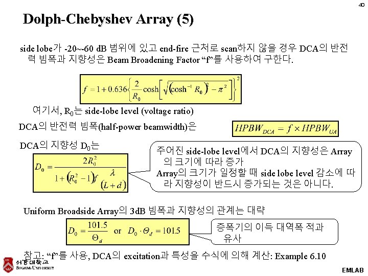
 m차 Chebyshev Polynomial의 일부분이 Visible Range로 설정됨 소자간 거리 d의")
39 Dolph-Chebyshev Array (4) m차 Chebyshev Polynomial의 일부분이 Visible Range로 설정됨 소자간 거리 d의 크기에 따라 Visible Range가 변 한다. 단, z 0는 항상 주빔으로 포함. 어떤 Minor lobe도 주어진 Level을 넘지 않을 조건 9차 Chebyshev Polinomial의 Magnitude 10 소자 DCA의 Array Factor Pattern EMLAB
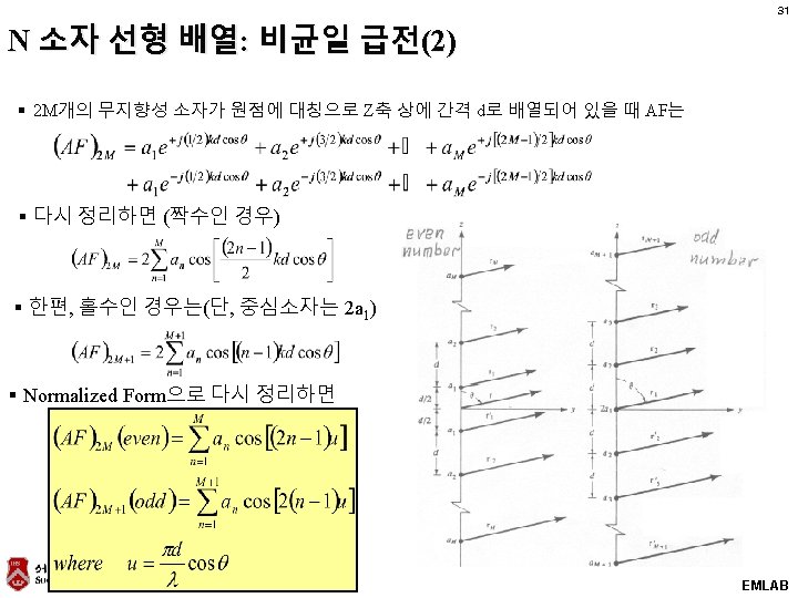
 모든 배열 소자가 동일한 급전 계수를 갖는 경우 즉, 이면")
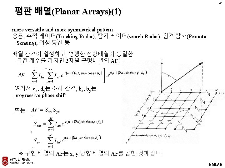
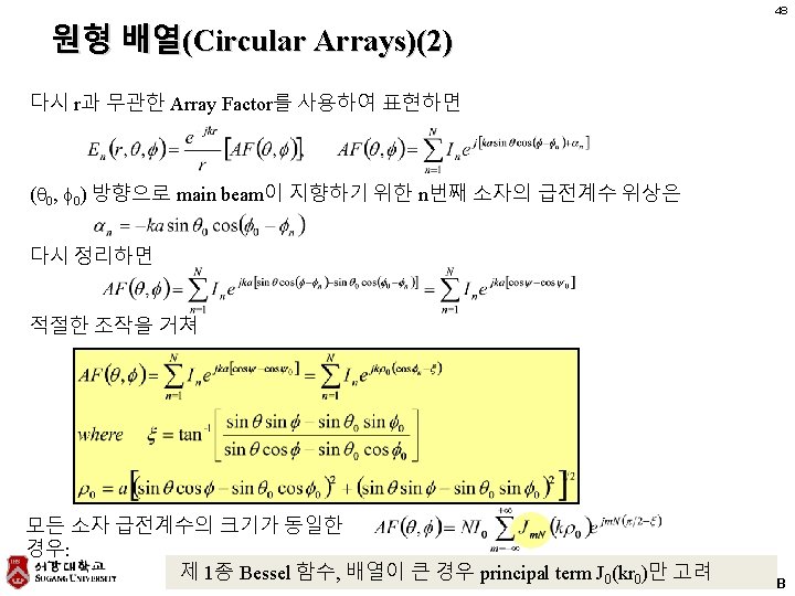
42 Planar Arrays (2) 모든 배열 소자가 동일한 급전 계수를 갖는 경우 즉, 이면 Normalized Array Factor는 Major Lobe와 Grating Lobe는 Main Beam을 (θ 0, φ0)방향으로 지향하기 위한 Progressive phase shift는 EMLAB
 Major Lobe와 Grating Lobe는 또는 윗 식으로부터 θ, φ를 구하면")
43 Planar Arrays (3) Major Lobe와 Grating Lobe는 또는 윗 식으로부터 θ, φ를 구하면 EMLAB
 EMLAB")
44 Planar Arrays (4) EMLAB
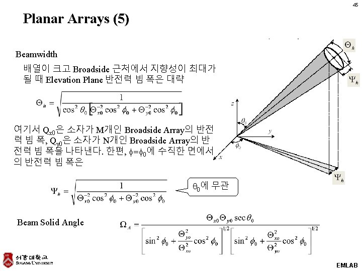
 지향성(Directivity) 배열이 크고 Broadside 근처에서 지향성이 최대가 될 때 지향성의")
46 Planar Arrays (6) 지향성(Directivity) 배열이 크고 Broadside 근처에서 지향성이 최대가 될 때 지향성의 근사식은 배열의 Projected Area 감소 효과 지향성을 Beam Solid Angle로 나타낸 근사식 Example & Design Consideration EMLAB
 : Rotman Lens 49 EMLAB")
Beamforming Approaches (1) : Rotman Lens 49 EMLAB

Pictures of Rotman Lens 50 EMLAB
 Circuit Beamformer Blass Matrix Butler Matrix EMLAB")
51 Beamforming Approaches (1) Circuit Beamformer Blass Matrix Butler Matrix EMLAB
 Digital Beamformer (DBF) or ce en fer th a In")
52 Beamforming Approaches (2) Digital Beamformer (DBF) or ce en fer th a In ion ltip ect dir mu n sig al LPF d si Desire on directi A/D LPF A/D gnal Digital Signal Processing (Amplitude & Phase) ~ EMLAB

53 Antenna beam synthesis EMLAB
 v - This method is used to determine the excitation distribution")
Fourier Transform Method(1) v - This method is used to determine the excitation distribution of a continuous or a discrete source antenna system for a given desired pattern v i) Line-Source v v v 54 The excitation phase constant of the source ii) For uniform current distribution, EMLAB
 v v Transform Pair v v v Fourier Transform Inverse")
55 Fourier Transform Method(2) v v Transform Pair v v v Fourier Transform Inverse Fourier Transform - The above equation relates the excitation distribution of continuous source to its far-field space factor - The approximate source distribution is given by EMLAB
 v Desired pattern v v v v Approximate pattern -")
56 Fourier Transform Method(3) v Desired pattern v v v v Approximate pattern - The approximate pattern is used to represent, within certain error, the desired pattern - Over all values of ζ, the synthesized approximate pattern SF(θ)_a yields the least mean square error or deviation from the desired pattern SF(θ)_d - However that criterion is not satisfied when the values of ζ are restricted only in the visible region(!!!) Ex. 7. 2 finite range of zeta EMLAB

57 EMLAB
 v iii) Linear Array If the reference point is taken")
58 Fourier Transform Method(4) v iii) Linear Array If the reference point is taken at the physical center of the array, v i) Odd Number of Elements (N=2 M+1) v ii) Odd Number of Elements (N=2 M) v The elements are placed at v v (for an even number) (for an odd number) EMLAB
 v - If AF represents the desired array")
59 7. 4 Fourier Transform Method(5) v - If AF represents the desired array factor, the excitation coefficients of the array can be obtained by the Fourier formula v i) Odd Number of Elements (N=2 M+1) v v ii) Odd Number of Elements (N=2 M) v - Fig. 7 -6(b) : Line-source, Fig. 7 -7 : Linear Array v - Discrete element linear arrays only approximate continuous line-sources - Their patterns shown in Fig. 7. 7 do not approximate as well the desired pattern as the corresponding patterns of the line-source distribution v v EMLAB

60 EMLAB
 v - This method is accomplished by sampling the desired pattern")
61 Woodward-Lawson Method(1) v - This method is accomplished by sampling the desired pattern at various discrete locations Angles where the desired pattern is sampled i) Line-Source v Each Current Distribution : v v v Total current : v v The corresponding field pattern : (= composing function) v v Total pattern : The maximum of each individual term occurs when θ = θm EMLAB

62 EMLAB
 v The characteristics of space factor : - When one term")
63 Woodward-Lawson Method(2) v The characteristics of space factor : - When one term attains its maximum value at its sample at theta=theta_m, all other terms of above equation which are associated with the other samples are zero at theta=theta_m - In other words, all sampling terms(composing functions) are zero at all sampling points other than at their own - Thus at each sampling point the total field is equal to that of the sample v - To faithfully reconstruct the desired pattern, v (separation) v (location) EMLAB
 v ii) Linear Array (to synthesize discrete linear arrays) v v The")
Woodward-Lawson Method(3) v ii) Linear Array (to synthesize discrete linear arrays) v v The pattern of each sample (assuming that the array is equal to the length of line source) v The array factor(as a superposition) v The excitation coefficients of the array elements at the sample points v v 64 the value of the desired array factor The sample points EMLAB
 v - Comparison between the Fourier-Transform Method and Woodward-Lawson Method v")
65 Woodward-Lawson Method(4) v - Comparison between the Fourier-Transform Method and Woodward-Lawson Method v i) Fourier Transform Method - v - - yields reconstructed patterns whose mean-square error(or deviation) from the desired pattern is a minimum - is best suited for reconstruction of desired patterns which are analytically simple and which allow the integrations to be performed in closed form ii) Woodward-Lawson Method - reconstructs patterns whose values at the sampled points are identical to the ones of the desired pattern it does not have any control of the pattern between the sample points it does not yield a pattern with least mean-square deviation - - is more flexible and it can be used to synthesize any desired pattern. - - it can even be used to reconstruct patterns which cannot be expressed analytically - EMLAB
- Slides: 65