1 Advanced Digital Signal Processing Office 723 TEL

1 Advanced Digital Signal Processing 高等數位訊號處理 授課者： 丁 建 均 Office：明達館 723室, TEL： 33669652 E-mail: djj 1@ms 63. hinet. net , djj@cc. ee. ntu. edu. tw 課程網頁：http: //djj. ee. ntu. edu. tw/ADSP. htm 歡迎大家來修課，也歡迎有問題時隨時聯絡！

Tutorial 可供選擇的題目(共 18 個，可以略做修改) (1) Adaptive Wiener Filter (2) Bilateral Filter (3) Tone Analysis (4) Image Deblurring (5) Sharpness Measurement for Images (6) Image Compression Based on Structural Similarity (SSIM) (7) Medical Image Compression (8) JBIG and Binary Image Compression (9) Arithmetic Coding (10) Structure Similarity (加強) (11) Jacket Transform (12) Integer Transform (加強) (續) 5

Tutorial 可供選擇的題目(可以略做修改) (13) Fermat and Mersenne Numbers (14) Non-Linear Time Variant System Analysis (加強) (15) Support Vector Machine (16) 3 -D Accelerometer Signal Analysis (17) Nonuniform Sampling (18) Eletromyography (EMG ) Signal Analysis 6

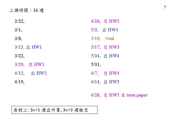
7 上課時間： 16 週 2/22, 4/26, 交 HW 2 3/1, 5/3, 出 HW 3 3/8, 5/10, 3/15, 出 HW 1 5/17, 交 HW 3 3/22, 5/24, 出 HW 4 3/29, 交 HW 1 5/31, 4/12, 6/7, 出 HW 2 4/19, Oral 交 HW 4 6/14, 出 HW 5 6/28, 交 HW 5 及 term paper 原則上: 3 n+1 週出作業, 3 n+3 週繳交

10 Question: Why should we use the Fourier transform?

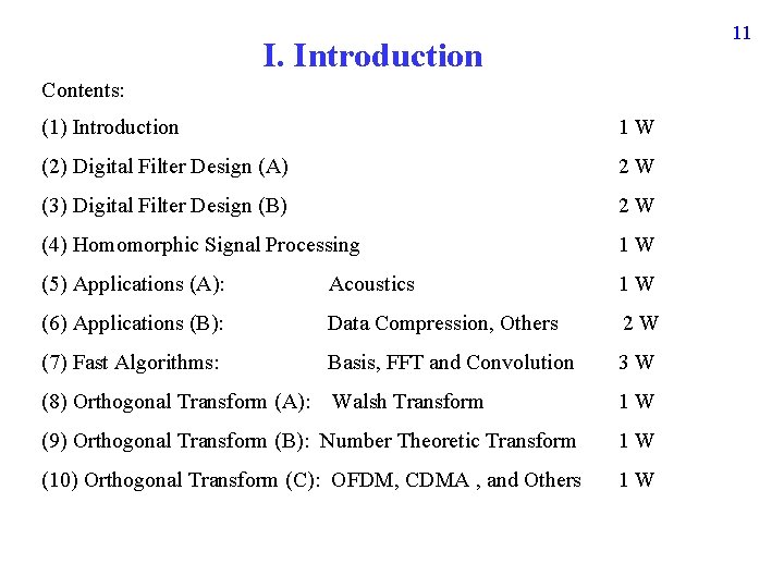
11 I. Introduction Contents: (1) Introduction 1 W (2) Digital Filter Design (A) 2 W (3) Digital Filter Design (B) 2 W (4) Homomorphic Signal Processing 1 W (5) Applications (A): Acoustics 1 W (6) Applications (B): Data Compression, Others 2 W (7) Fast Algorithms: Basis, FFT and Convolution 3 W (8) Orthogonal Transform (A): Walsh Transform 1 W (9) Orthogonal Transform (B): Number Theoretic Transform 1 W (10) Orthogonal Transform (C): OFDM, CDMA , and Others 1 W

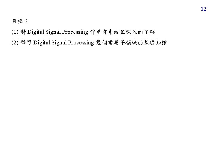
12 目標： (1) 對 Digital Signal Processing 作更有系統且深入的了解 (2) 學習 Digital Signal Processing 幾個重要子領域的基礎知識

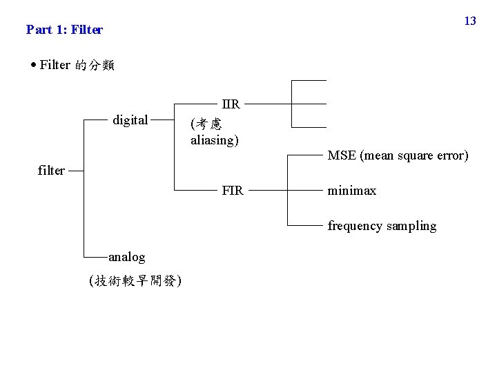
13 Part 1: Filter 的分類 digital IIR (考慮 aliasing) MSE (mean square error) filter FIR minimax frequency sampling analog (技術較早開發)

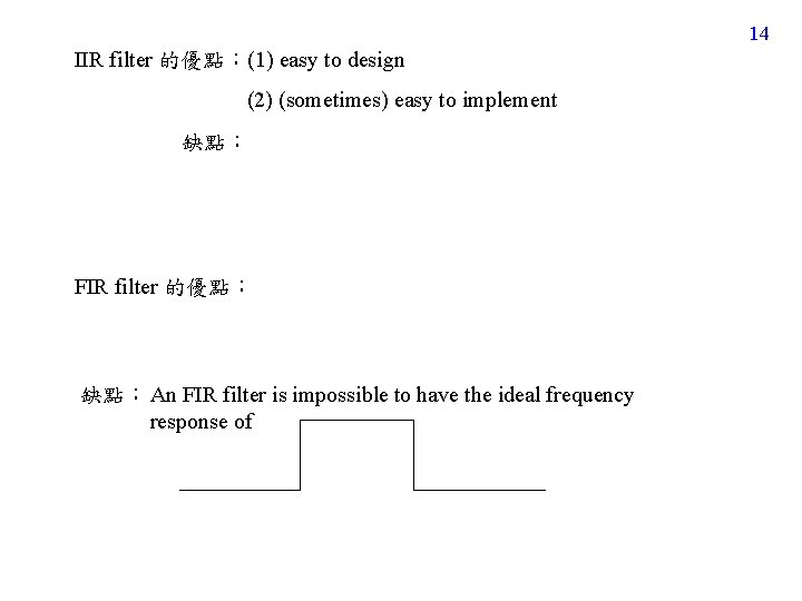
14 IIR filter 的優點：(1) easy to design (2) (sometimes) easy to implement 缺點： FIR filter 的優點： 缺點： An FIR filter is impossible to have the ideal frequency response of

Part 2: Homomorphic Signal Processing 15 概念：把 convolution 變成 addition Part 3: Applications of DSP filter design, data compression (image, video, text), acoustics (speech, music), image analysis (structural similarity, sharpness), 3 D accelerometer

Part 4: Fast Algorithms Basic Implementation Techniques Example: one complex number multiplication = ? Real number multiplication. Trade-off: “Multiplication” takes longer than “addition” 16

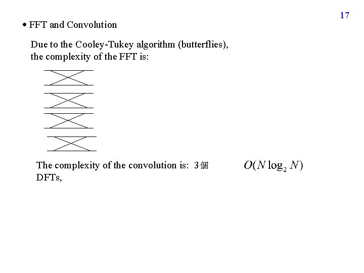
FFT and Convolution Due to the Cooley-Tukey algorithm (butterflies), the complexity of the FFT is: The complexity of the convolution is: 3個 DFTs, 17

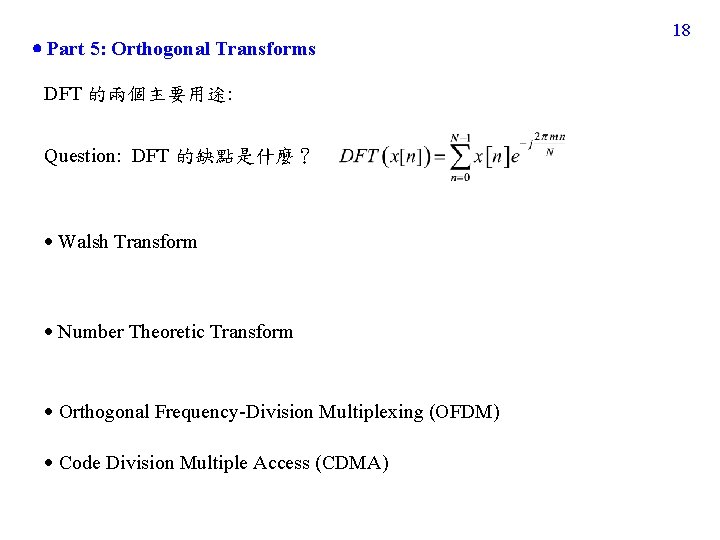
Part 5: Orthogonal Transforms DFT 的兩個主要用途: Question: DFT 的缺點是什麼？ Walsh Transform Number Theoretic Transform Orthogonal Frequency-Division Multiplexing (OFDM) Code Division Multiple Access (CDMA) 18

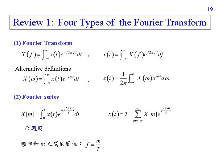
19 Review 1: Four Types of the Fourier Transform (1) Fourier Transform , Alternative definitions , (2) Fourier series T: 週期 頻率和 m 之間的關係：

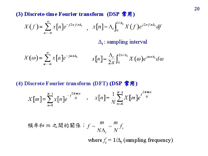
(3) Discrete-time Fourier transform (DSP 常用) , t : sampling interval (4) Discrete Fourier transform (DFT) (DSP 常用) , 頻率和 m 之間的關係： where fs = 1/ t (sampling frequency) 20

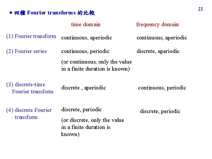
21 四種 Fourier transforms 的比較 time domain (1) Fourier transform continuous, aperiodic (2) Fourier series continuous, periodic frequency domain continuous, aperiodic discrete, aperiodic (or continuous, only the value in a finite duration is known) (3) discrete-time Fourier transform (4) discrete Fourier transform discrete , aperiodic continuous, periodic discrete, periodic (or discrete, only the value in a finite duration is known)

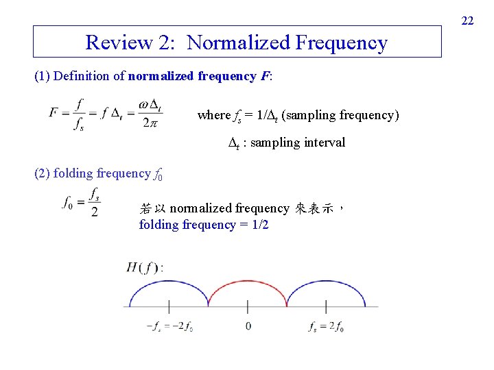
22 Review 2: Normalized Frequency (1) Definition of normalized frequency F: where fs = 1/ t (sampling frequency) t : sampling interval (2) folding frequency f 0 若以 normalized frequency 來表示， folding frequency = 1/2

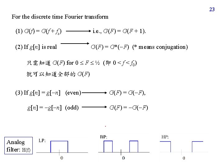
23 For the discrete time Fourier transform (1) G(f) = G(f + fs) i. e. , G(F) = G(F + 1). (2) If g[n] is real G(F) = G*( F) (* means conjugation) 只需知道 G(F) for 0 F ½ (即 0 < f 0) 就可以知道全部的 G(F) (3) If g[n] = g[ n] (even) g[n] = g[ n] (odd) Analog filter: H(f) G(F) = G( F), G(F) = G( F)

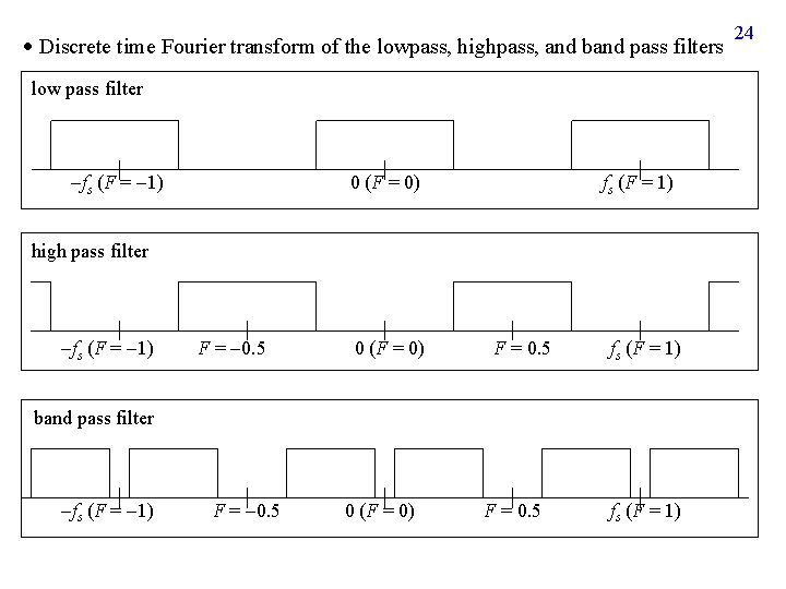
Discrete time Fourier transform of the lowpass, highpass, and band pass filters low pass filter fs (F = 1) 0 (F = 0) fs (F = 1) high pass filter fs (F = 1) F = 0. 5 0 (F = 0) F = 0. 5 fs (F = 1) band pass filter fs (F = 1) F = 0. 5 0 (F = 0) F = 0. 5 fs (F = 1) 24

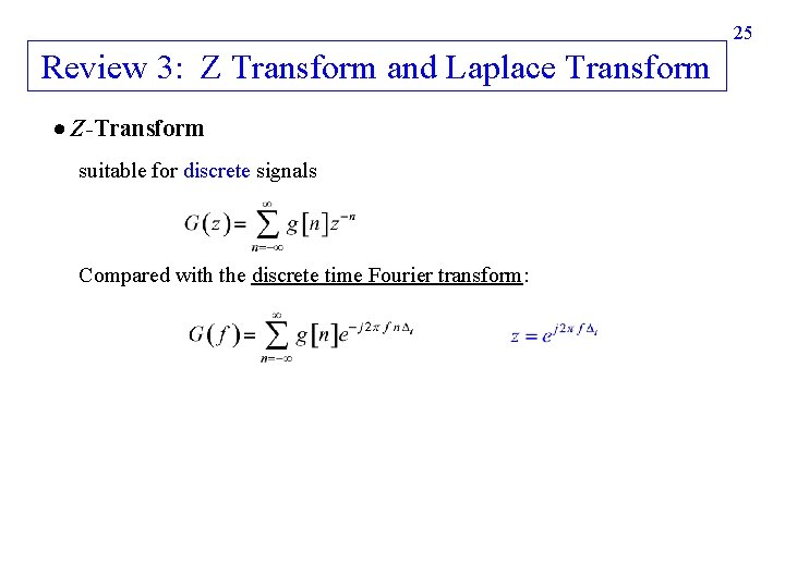
25 Review 3: Z Transform and Laplace Transform Z-Transform suitable for discrete signals Compared with the discrete time Fourier transform:

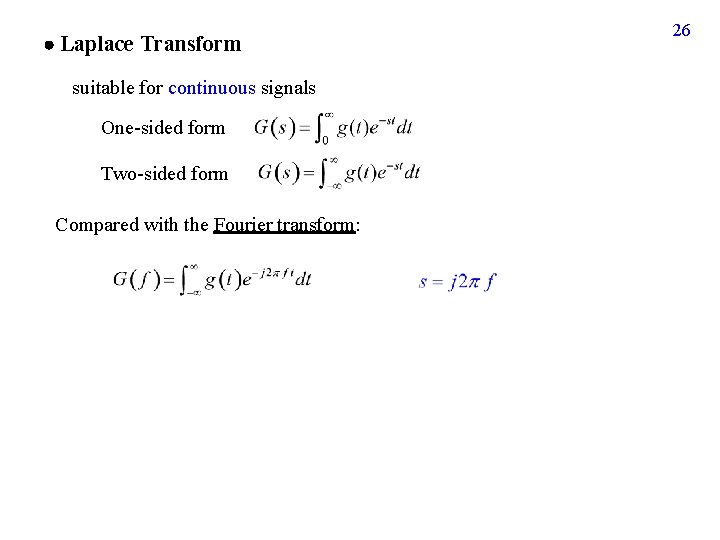
Laplace Transform suitable for continuous signals One-sided form Two-sided form Compared with the Fourier transform: 26

27 Review 4: IIR Filter Design Two types of digital filter: (1) IIR filter (infinite impulse response filter) (2) FIR filer (finite impulse response filer) There are 3 popular methods to design the IIR filter.

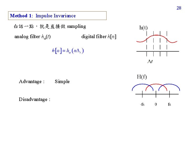
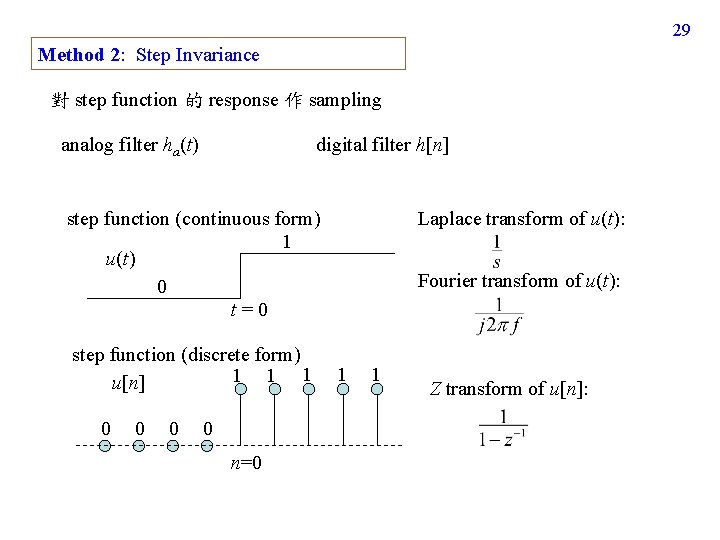
28 Method 1: Impulse Invariance 白話一點，就是直接做 sampling analog filter ha(t) Advantage : Disadvantage : digital filter h[n] Simple

29 Method 2: Step Invariance 對 step function 的 response 作 sampling analog filter ha(t) digital filter h[n] step function (continuous form) 1 u(t) 0 t=0 step function (discrete form) 1 1 1 u[n] 0 0 n=0 Laplace transform of u(t): Fourier transform of u(t): 1 1 Z transform of u[n]:

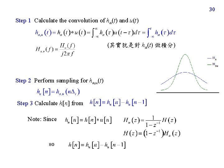
30 Step 1 Calculate the convolution of ha(t) and u(t) (其實就是對 ha(t) 做積分) Step 2 Perform sampling for ha, u(t) Step 3 Calculate h[n] from Note: Since so

31 Advantage of the step invariance method: Disadvantage of the step invariance method: 較為間接，設計上稍微複雜

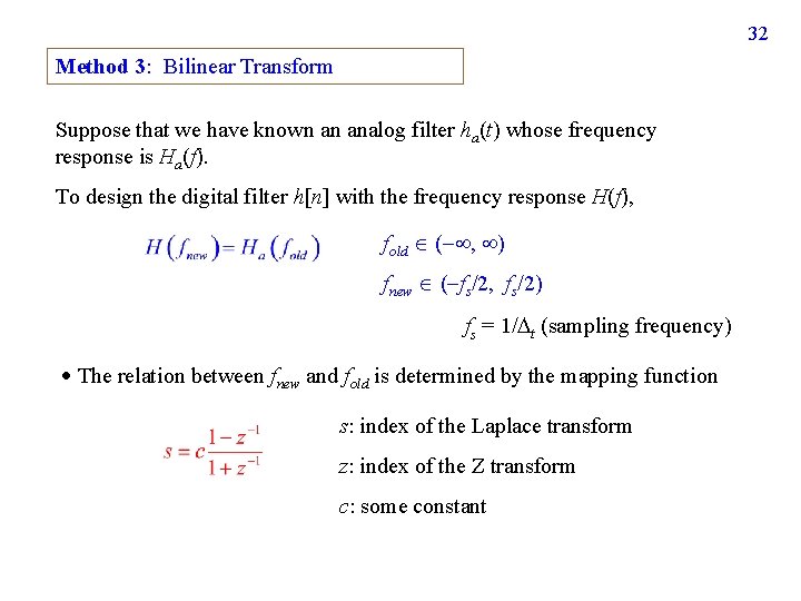
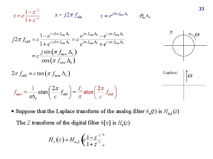
32 Method 3: Bilinear Transform Suppose that we have known an analog filter ha(t) whose frequency response is Ha(f). To design the digital filter h[n] with the frequency response H(f), fold ( , ) fnew ( fs/2, fs/2) fs = 1/ t (sampling frequency) The relation between fnew and fold is determined by the mapping function s: index of the Laplace transform z: index of the Z transform c: some constant

33 代入 Suppose that the Laplace transform of the analog filter ha(t) is Ha, L(s) The Z transform of the digital filter h[n] is Hz(z)

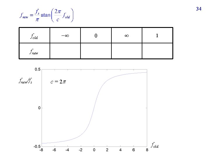
34 fold − 0 1 fnew/fs c = 2 fold

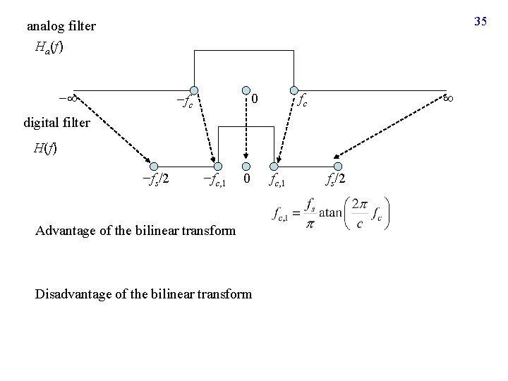
35 analog filter Ha(f) − 0 −fc fc digital filter H(f) −fs/2 −fc, 1 0 Advantage of the bilinear transform Disadvantage of the bilinear transform fc, 1 fs/2