1 A Dynamic Model of Aggregate 5 Demand

1 A Dynamic Model of Aggregate 5 Demand Aggregate Supply MACROECONOMICS N. Gregory Mankiw ® Power. Point Slides by Ron Cronovich © 2015 Worth Publishers, all rights reserved Fall 2014 update

IN THIS CHAPTER, YOU WILL LEARN: § how to incorporate dynamics into the AD-AS model we previously studied § how to use the dynamic AD-AS model to illustrate long-run economic growth § how to use the dynamic AD-AS model to trace out the effects over time of various shocks and policy changes on output, inflation, and other endogenous variables 1

Introduction § The dynamic model of aggregate demand aggregate supply gives us more insight into how the economy works in the short run. § It is a simplified version of a DSGE model, used in cutting-edge macroeconomic research. (DSGE = Dynamic, Stochastic, General Equilibrium) CHAPTER 15 Dynamic AD-AS Model 2

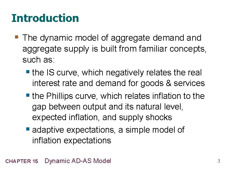
Introduction § The dynamic model of aggregate demand aggregate supply is built from familiar concepts, such as: § the IS curve, which negatively relates the real interest rate and demand for goods & services § the Phillips curve, which relates inflation to the gap between output and its natural level, expected inflation, and supply shocks § adaptive expectations, a simple model of inflation expectations CHAPTER 15 Dynamic AD-AS Model 3

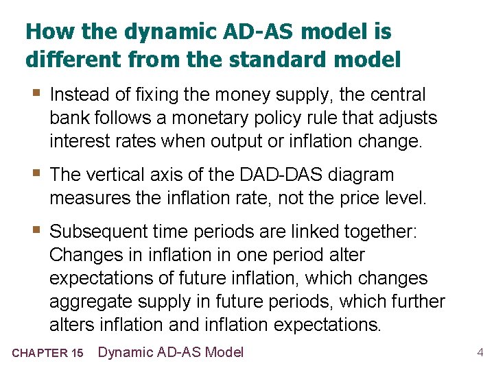
How the dynamic AD-AS model is different from the standard model § Instead of fixing the money supply, the central bank follows a monetary policy rule that adjusts interest rates when output or inflation change. § The vertical axis of the DAD-DAS diagram measures the inflation rate, not the price level. § Subsequent time periods are linked together: Changes in inflation in one period alter expectations of future inflation, which changes aggregate supply in future periods, which further alters inflation and inflation expectations. CHAPTER 15 Dynamic AD-AS Model 4

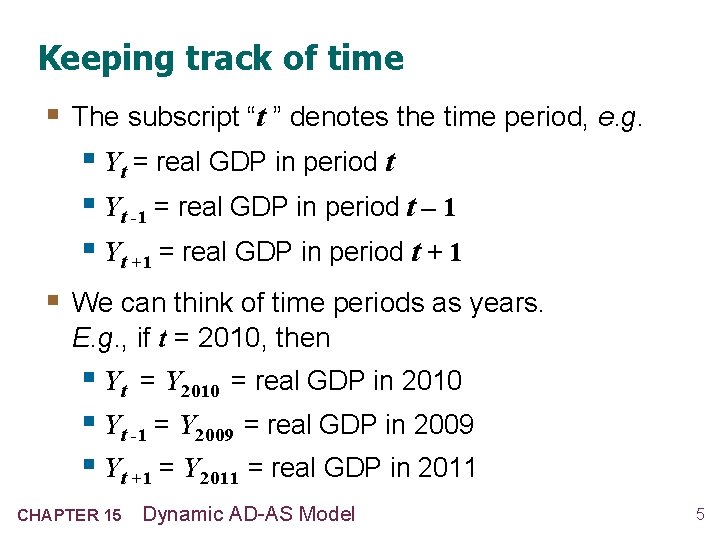
Keeping track of time § The subscript “t ” denotes the time period, e. g. § Yt = real GDP in period t § Yt -1 = real GDP in period t – 1 § Yt +1 = real GDP in period t + 1 § We can think of time periods as years. E. g. , if t = 2010, then § Yt = Y 2010 = real GDP in 2010 § Yt -1 = Y 2009 = real GDP in 2009 § Yt +1 = Y 2011 = real GDP in 2011 CHAPTER 15 Dynamic AD-AS Model 5

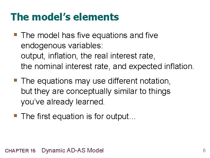
The model’s elements § The model has five equations and five endogenous variables: output, inflation, the real interest rate, the nominal interest rate, and expected inflation. § The equations may use different notation, but they are conceptually similar to things you’ve already learned. § The first equation is for output… CHAPTER 15 Dynamic AD-AS Model 6

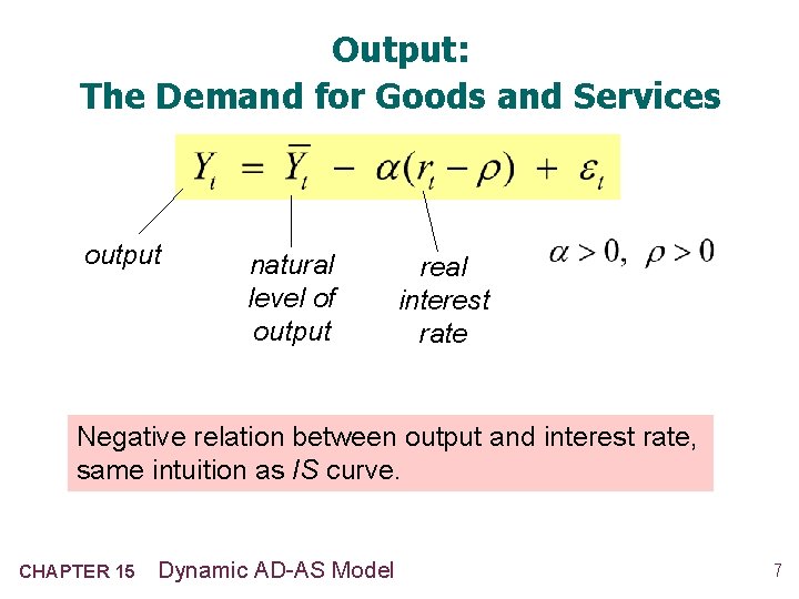
Output: The Demand for Goods and Services output natural level of output real interest rate Negative relation between output and interest rate, same intuition as IS curve. CHAPTER 15 Dynamic AD-AS Model 7

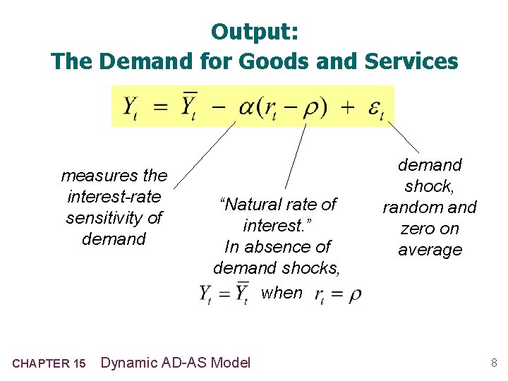
Output: The Demand for Goods and Services measures the interest-rate sensitivity of demand CHAPTER 15 “Natural rate of interest. ” In absence of demand shocks, when Dynamic AD-AS Model demand shock, random and zero on average 8

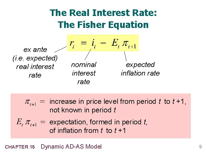
The Real Interest Rate: The Fisher Equation ex ante (i. e. expected) real interest rate nominal interest rate expected inflation rate increase in price level from period t to t +1, not known in period t expectation, formed in period t, of inflation from t to t +1 CHAPTER 15 Dynamic AD-AS Model 9

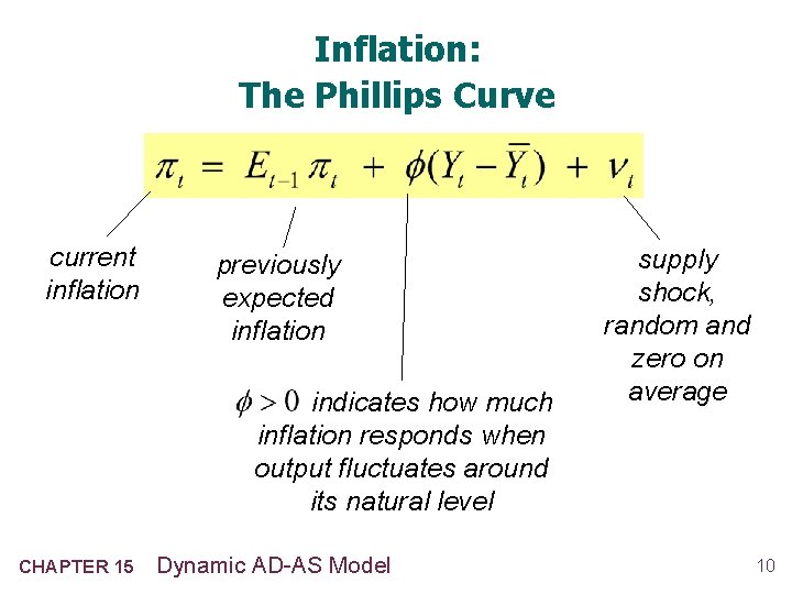
Inflation: The Phillips Curve current inflation previously expected inflation indicates how much inflation responds when output fluctuates around its natural level CHAPTER 15 Dynamic AD-AS Model supply shock, random and zero on average 10

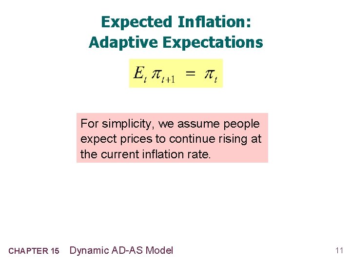
Expected Inflation: Adaptive Expectations For simplicity, we assume people expect prices to continue rising at the current inflation rate. CHAPTER 15 Dynamic AD-AS Model 11

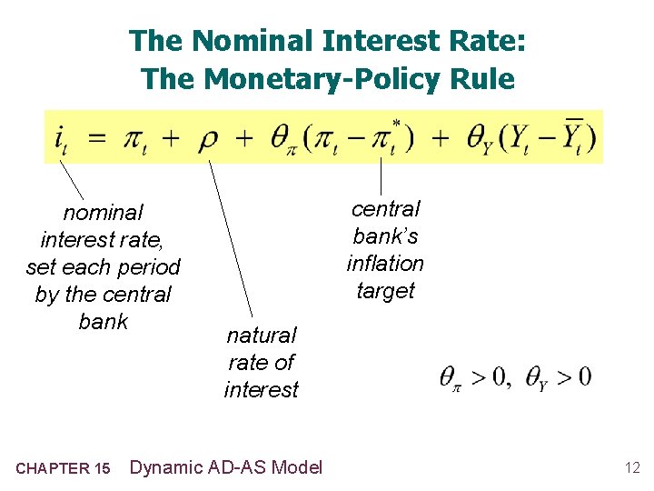
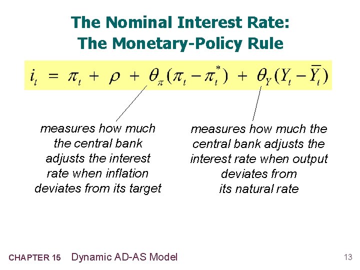
The Nominal Interest Rate: The Monetary-Policy Rule nominal interest rate, set each period by the central bank CHAPTER 15 central bank’s inflation target natural rate of interest Dynamic AD-AS Model 12

The Nominal Interest Rate: The Monetary-Policy Rule measures how much the central bank adjusts the interest rate when inflation deviates from its target CHAPTER 15 Dynamic AD-AS Model measures how much the central bank adjusts the interest rate when output deviates from its natural rate 13

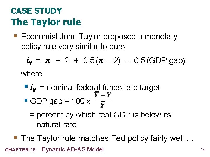
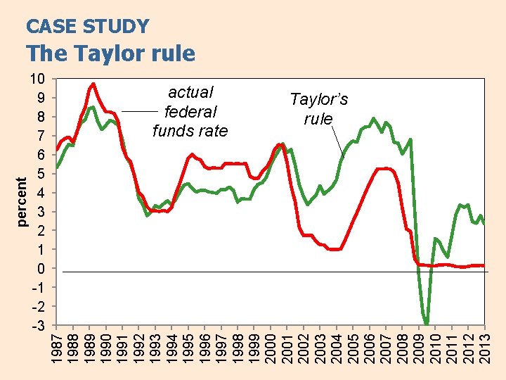
CASE STUDY The Taylor rule § Economist John Taylor proposed a monetary policy rule very similar to ours: iff = π + 2 + 0. 5 (π – 2) – 0. 5 (GDP gap) where § iff = nominal federal funds rate target § GDP gap = 100 x = percent by which real GDP is below its natural rate § The Taylor rule matches Fed policy fairly well. … CHAPTER 15 Dynamic AD-AS Model 14

percent 10 9 8 7 6 5 4 3 2 1 0 -1 -2 -3 1987 1988 1989 1990 1991 1992 1993 1994 1995 1996 1997 1998 1999 2000 2001 2002 2003 2004 2005 2006 2007 2008 2009 2010 2011 2012 2013 CASE STUDY The Taylor rule actual federal funds rate Taylor’s rule

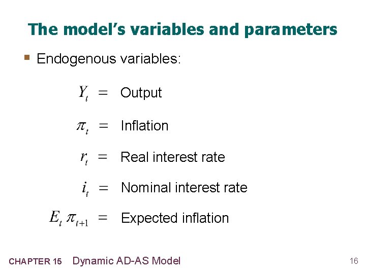
The model’s variables and parameters § Endogenous variables: Output Inflation Real interest rate Nominal interest rate Expected inflation CHAPTER 15 Dynamic AD-AS Model 16

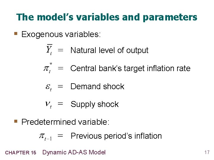
The model’s variables and parameters § Exogenous variables: Natural level of output Central bank’s target inflation rate Demand shock Supply shock § Predetermined variable: Previous period’s inflation CHAPTER 15 Dynamic AD-AS Model 17

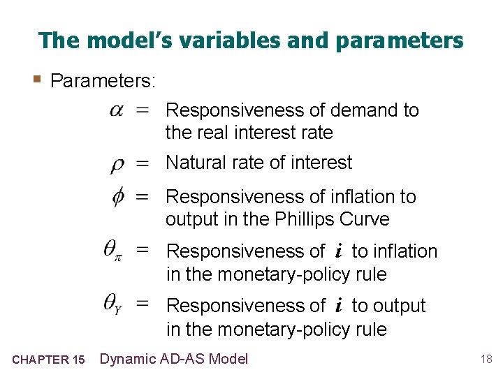
The model’s variables and parameters § Parameters: Responsiveness of demand to the real interest rate Natural rate of interest Responsiveness of inflation to output in the Phillips Curve Responsiveness of i to inflation in the monetary-policy rule Responsiveness of i to output in the monetary-policy rule CHAPTER 15 Dynamic AD-AS Model 18

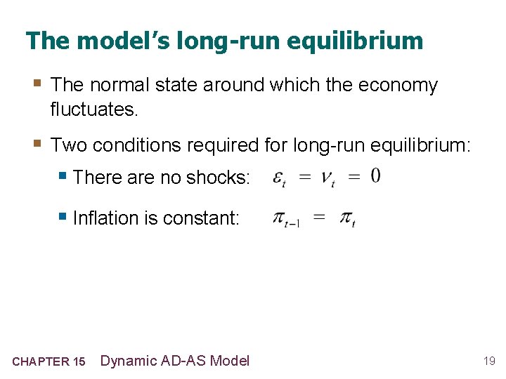
The model’s long-run equilibrium § The normal state around which the economy fluctuates. § Two conditions required for long-run equilibrium: § There are no shocks: § Inflation is constant: CHAPTER 15 Dynamic AD-AS Model 19

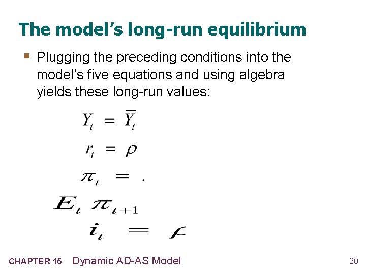
The model’s long-run equilibrium § Plugging the preceding conditions into the model’s five equations and using algebra yields these long-run values: CHAPTER 15 Dynamic AD-AS Model 20

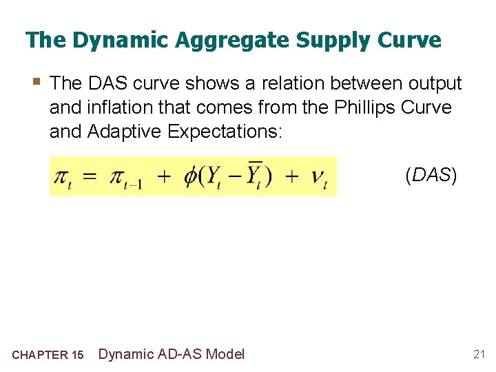
The Dynamic Aggregate Supply Curve § The DAS curve shows a relation between output and inflation that comes from the Phillips Curve and Adaptive Expectations: (DAS) CHAPTER 15 Dynamic AD-AS Model 21

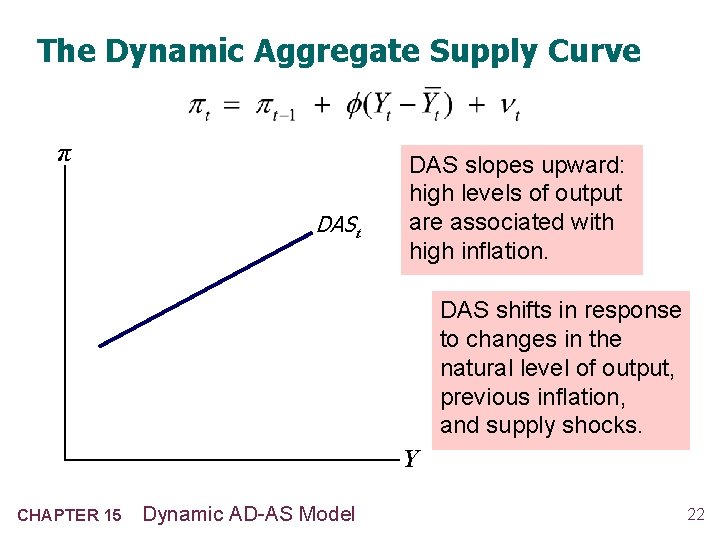
The Dynamic Aggregate Supply Curve π DASt DAS slopes upward: high levels of output are associated with high inflation. DAS shifts in response to changes in the natural level of output, previous inflation, and supply shocks. Y CHAPTER 15 Dynamic AD-AS Model 22

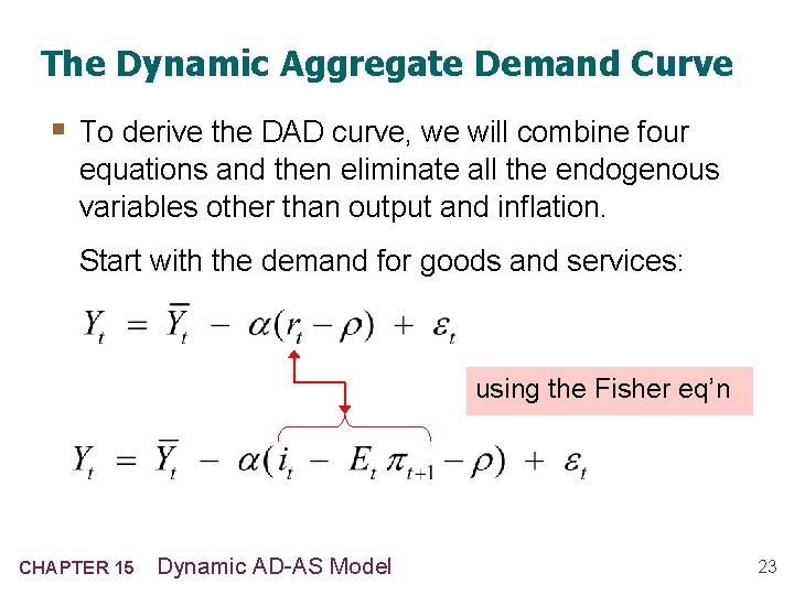
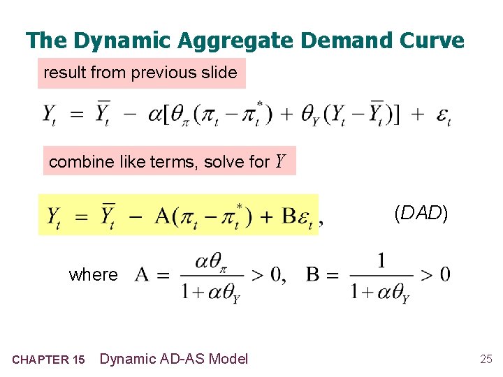
The Dynamic Aggregate Demand Curve § To derive the DAD curve, we will combine four equations and then eliminate all the endogenous variables other than output and inflation. Start with the demand for goods and services: using the Fisher eq’n CHAPTER 15 Dynamic AD-AS Model 23

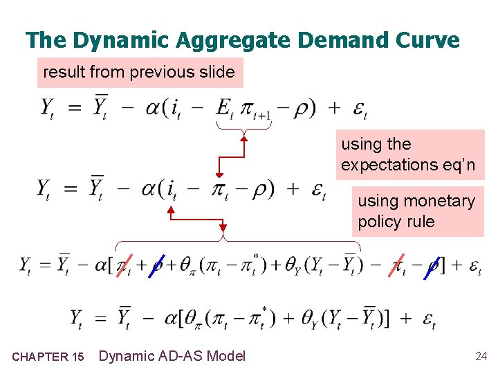
The Dynamic Aggregate Demand Curve result from previous slide using the expectations eq’n using monetary policy rule CHAPTER 15 Dynamic AD-AS Model 24

The Dynamic Aggregate Demand Curve result from previous slide combine like terms, solve for Y (DAD) where CHAPTER 15 Dynamic AD-AS Model 25

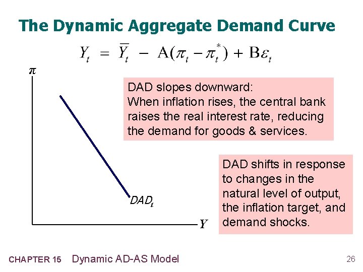
The Dynamic Aggregate Demand Curve π DAD slopes downward: When inflation rises, the central bank raises the real interest rate, reducing the demand for goods & services. DADt Y CHAPTER 15 Dynamic AD-AS Model DAD shifts in response to changes in the natural level of output, the inflation target, and demand shocks. 26

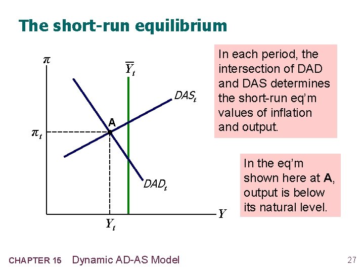
The short-run equilibrium π Yt DASt πt A In each period, the intersection of DAD and DAS determines the short-run eq’m values of inflation and output. DADt Yt CHAPTER 15 Dynamic AD-AS Model Y In the eq’m shown here at A, output is below its natural level. 27

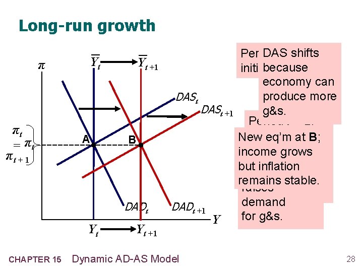
Long-run growth π Yt Yt +1 DASt πt = πt πt + 1 A B DADt Yt CHAPTER 15 DASt +1 DADt +1 Yt +1 Dynamic AD-AS Model Y DAS Period t: shifts initialbecause eq’m at A economy can produce more g&s. Period t + 1: Long-run New eq’m at B; DAD shifts growthgrows income because increases but inflation the higher income naturalstable. rate remains raises of output. demand for g&s. 28

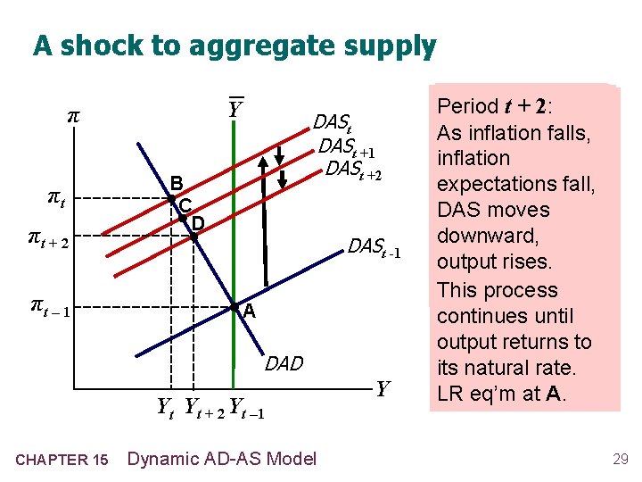
A shock to aggregate supply Y π πt πt + 2 πt – 1 DASt +1 DASt +2 B C D DASt -1 A DAD Yt Yt + 2 Yt – 1 CHAPTER 15 Dynamic AD-AS Model Y Periodtt+ : – 121: : Period initial eq’m at A Supply shock As inflation falls, (νover > 0)(shifts is ν = 0) inflation DAS upward; but DAS doesfall, not expectations inflation rises, return to its initial DAS moves central bank position due to downward, responds by higher inflation output rises. raising real expectations. This process interest rate, continues until outputreturns falls. to output its natural rate. LR eq’m at A. 29

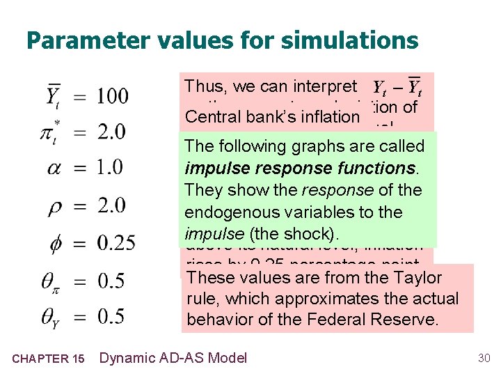
Parameter values for simulations Thus, we can interpret Yt – Yt as the percentage deviation of Central bank’s inflation output from its natural level. target is 2 percent. A 1 -percentage-point increase The following graphs are called in the realresponse interest rate reduces impulse functions. outputshow demand by 1 percent of They the response of the The natural rate of interest is its natural level. endogenous 2 percent. variables to the When output is 1 percent impulse (the shock). above its natural level, inflation rises by 0. 25 percentage point. These values are from the Taylor rule, which approximates the actual behavior of the Federal Reserve. CHAPTER 15 Dynamic AD-AS Model 30

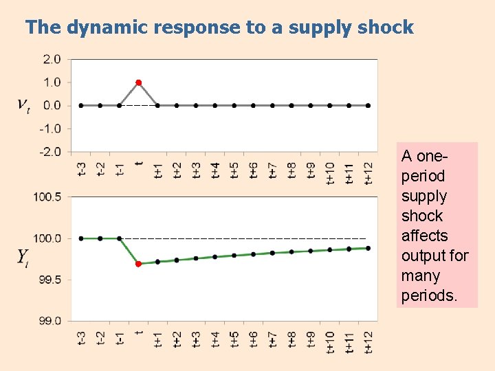
The dynamic response to a supply shock A oneperiod supply shock affects output for many periods.

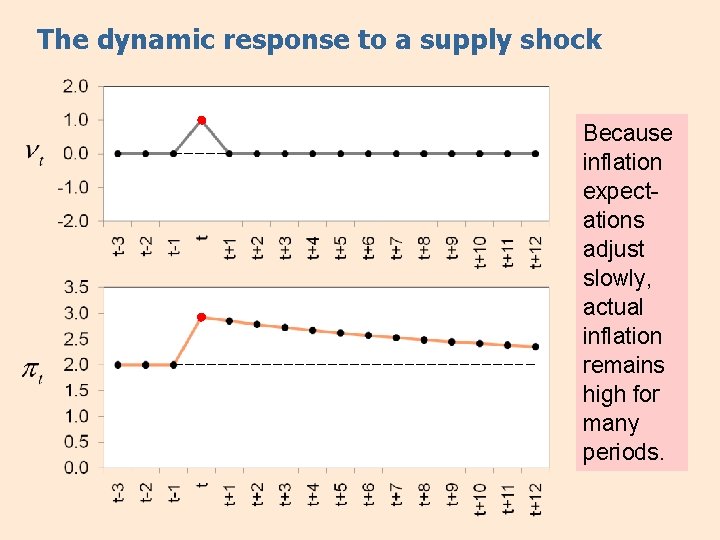
The dynamic response to a supply shock Because inflation expectations adjust slowly, actual inflation remains high for many periods.

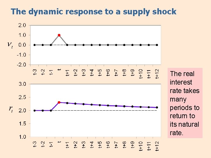
The dynamic response to a supply shock The real interest rate takes many periods to return to its natural rate.

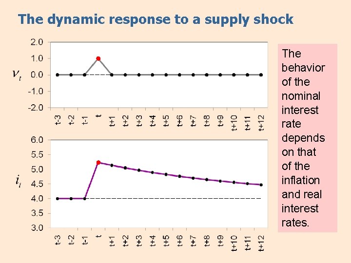
The dynamic response to a supply shock The behavior of the nominal interest rate depends on that of the inflation and real interest rates.

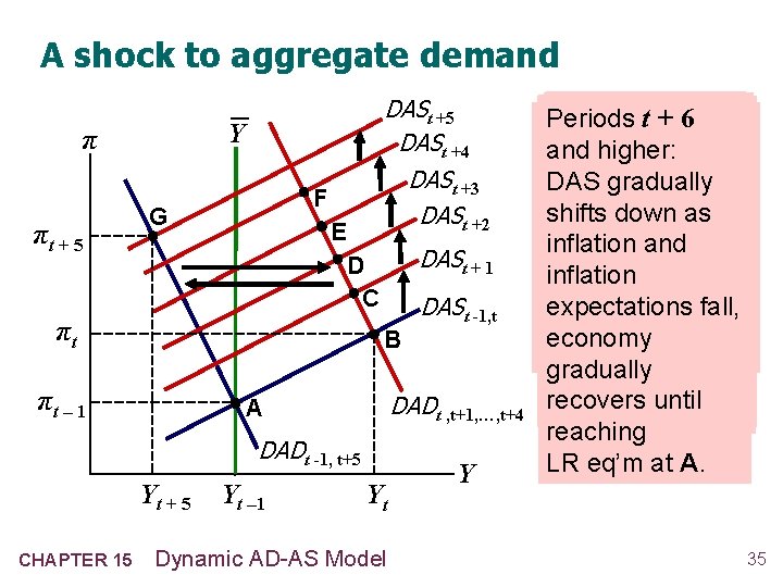
A shock to aggregate demand Y π πt + 5 DASt +4 DASt +3 DASt +2 F G E DASt + 1 D C πt DASt -1, t B πt – 1 DADt , t+1, …, t+4 A DADt -1, t+5 Yt + 5 CHAPTER 15 Yt – 1 Yt Dynamic AD-AS Model Y : t–+1+ Periods Period 516: : : 2 Periods Period ttt+t+ Positive initial at Ain and higher: DAS is 4 eq’m higher Higher inflation to t+ : demand shock DAS togradually higher tdue raised inflation Higher inflation (ε previous > 0) shifts down inflation in as in expectations ADt +to 1 the right; inflation and preceding period, period for , raises output and up. inflation but demand inflation shifting DAS inflation rise. expectations fall, shock ends and expectations, Inflation rises economy DAD to shiftsreturns DAS up. more, output falls. gradually its initial position. Inflation rises, recovers until Eq’m atfalls. G. output reaching LR eq’m at A. 35

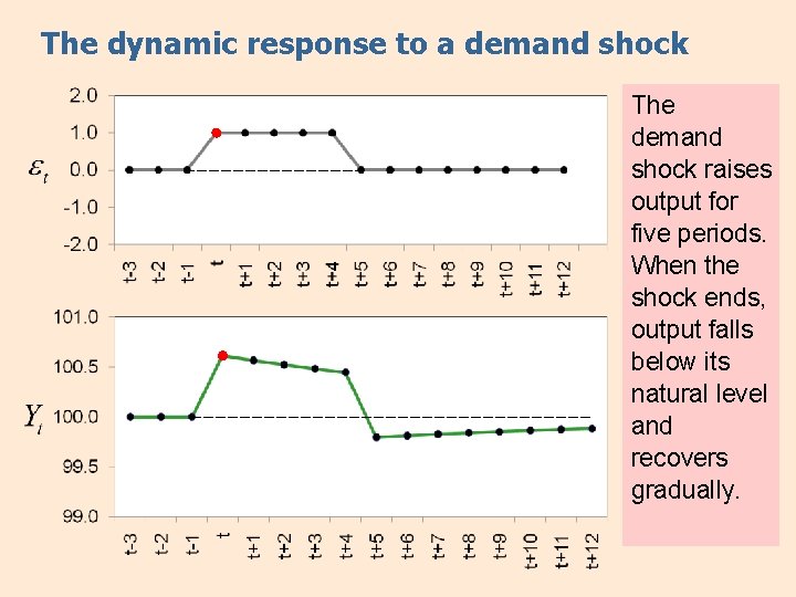
The dynamic response to a demand shock The demand shock raises output for five periods. When the shock ends, output falls below its natural level and recovers gradually.

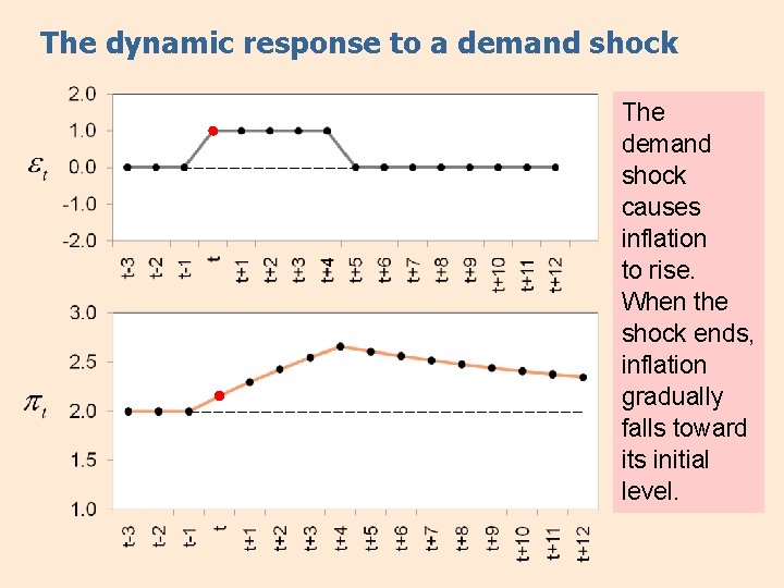
The dynamic response to a demand shock The demand shock causes inflation to rise. When the shock ends, inflation gradually falls toward its initial level.

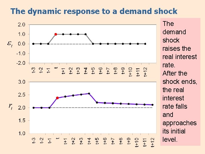
The dynamic response to a demand shock The demand shock raises the real interest rate. After the shock ends, the real interest rate falls and approaches its initial level.

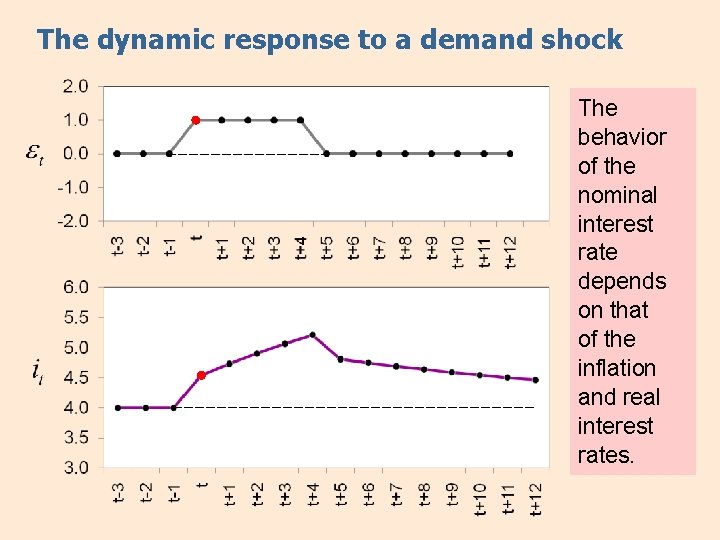
The dynamic response to a demand shock The behavior of the nominal interest rate depends on that of the inflation and real interest rates.

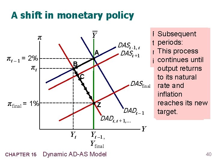
A shift in monetary policy Y π πt – 1 = 2% πt A B C πfinal = 1% Z Subsequent Period t t–t+ Period : 1: 1 : Period periods: target inflation The fall in πt Central bank DASt -1, t This lowers rate π*process = target 2%, reduced DASt +1 continues until inflation initial at A to π*eq’m = 1%, output expectations raises returns real to its for t +natural 1, shifting interest rate, DASfinal DAS rate downward. shiftsand DAD inflation Output rises, leftward. reaches its new inflation falls. Output and DADt – 1 target. inflation fall. DADt, t + 1, … Yt CHAPTER 15 Yt – 1 , Yfinal Dynamic AD-AS Model Y 40

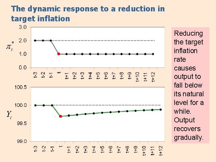
The dynamic response to a reduction in target inflation Reducing the target inflation rate causes output to fall below its natural level for a while. Output recovers gradually.

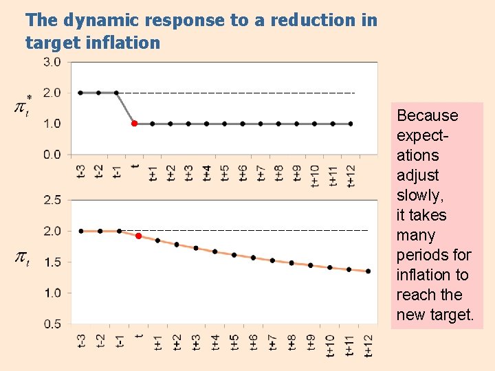
The dynamic response to a reduction in target inflation Because expectations adjust slowly, it takes many periods for inflation to reach the new target.

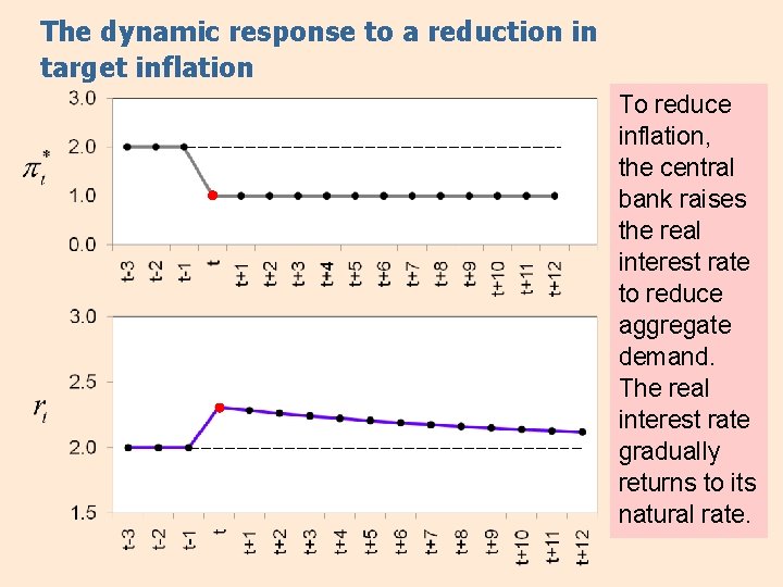
The dynamic response to a reduction in target inflation To reduce inflation, the central bank raises the real interest rate to reduce aggregate demand. The real interest rate gradually returns to its natural rate.

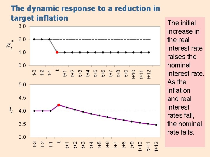
The dynamic response to a reduction in target inflation The initial increase in the real interest rate raises the nominal interest rate. As the inflation and real interest rates fall, the nominal rate falls.

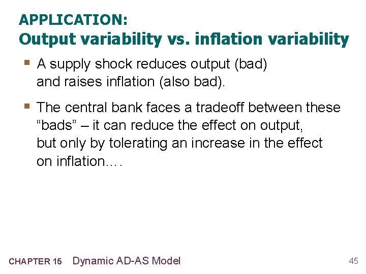
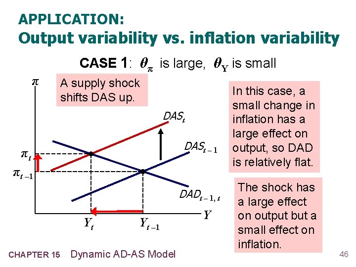
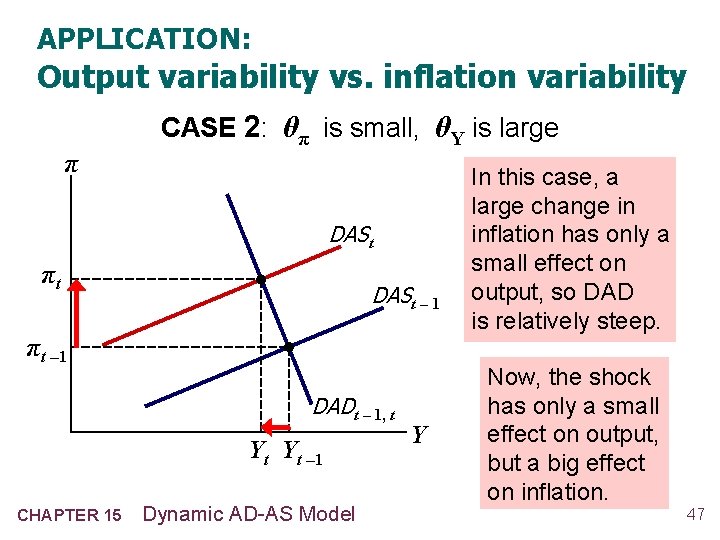
APPLICATION: Output variability vs. inflation variability § A supply shock reduces output (bad) and raises inflation (also bad). § The central bank faces a tradeoff between these “bads” – it can reduce the effect on output, but only by tolerating an increase in the effect on inflation…. CHAPTER 15 Dynamic AD-AS Model 45

APPLICATION: Output variability vs. inflation variability π CASE 1: θπ is large, θY is small A supply shock shifts DAS up. DASt – 1 πt πt – 1 DADt – 1, t Yt CHAPTER 15 Yt – 1 Dynamic AD-AS Model Y In this case, a small change in inflation has a large effect on output, so DAD is relatively flat. The shock has a large effect on output but a small effect on inflation. 46

APPLICATION: Output variability vs. inflation variability π CASE 2: θπ is small, θY is large DASt πt DASt – 1 πt – 1 DADt – 1, t Yt Yt – 1 CHAPTER 15 Dynamic AD-AS Model Y In this case, a large change in inflation has only a small effect on output, so DAD is relatively steep. Now, the shock has only a small effect on output, but a big effect on inflation. 47

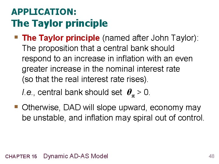
APPLICATION: The Taylor principle § The Taylor principle (named after John Taylor): The proposition that a central bank should respond to an increase in inflation with an even greater increase in the nominal interest rate (so that the real interest rate rises). I. e. , central bank should set θπ > 0. § Otherwise, DAD will slope upward, economy may be unstable, and inflation may spiral out of control. CHAPTER 15 Dynamic AD-AS Model 48

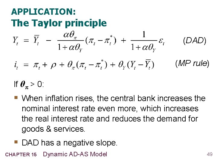
APPLICATION: The Taylor principle (DAD) (MP rule) If θπ > 0: § When inflation rises, the central bank increases the nominal interest rate even more, which increases the real interest rate and reduces the demand for goods & services. § DAD has a negative slope. CHAPTER 15 Dynamic AD-AS Model 49

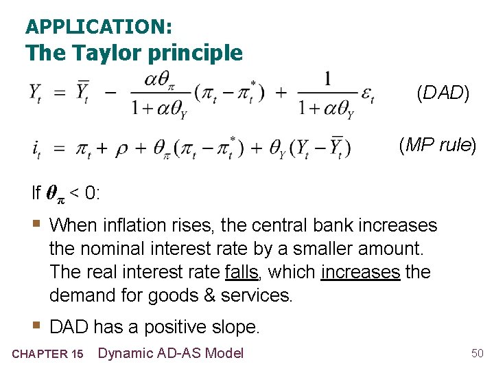
APPLICATION: The Taylor principle (DAD) (MP rule) If θπ < 0: § When inflation rises, the central bank increases the nominal interest rate by a smaller amount. The real interest rate falls, which increases the demand for goods & services. § DAD has a positive slope. CHAPTER 15 Dynamic AD-AS Model 50

APPLICATION: The Taylor principle § If DAD is upward-sloping and steeper than DAS, then the economy is unstable: output will not return to its natural level, and inflation will spiral upward (for positive demand shocks) or downward (for negative ones). § Estimates of θπ from published research: § θπ = – 0. 14 from 1960– 78, before Paul Volcker became Fed chairman. Inflation was high during this time, especially during the 1970 s. § θπ = 0. 72 during the Volcker and Greenspan years. Inflation was much lower during these years. CHAPTER 15 Dynamic AD-AS Model 51

CHAPTER SUMMARY § The DAD-DAS model combines five relationships: an IS-curve-like equation of the goods market, the Fisher equation, a Phillips curve equation, an equation for expected inflation, and a monetary policy rule. § The long-run equilibrium of the model is classical. Output and the real interest rate are at their natural levels, independent of monetary policy. The central bank’s inflation target determines inflation, expected inflation, and the nominal interest rate. 52

CHAPTER SUMMARY § The DAD-DAS model can be used to determine the immediate impact of any shock on the economy and can be used to trace out the effects of the shock over time. § The parameters of the monetary policy rule influence the slope of the DAS curve, so they determine whether a supply shock has a greater effect on output or inflation. Thus, the central bank faces a tradeoff between output variability and inflation variability. 53

CHAPTER SUMMARY § The DAD-DAS model assumes that the Taylor principle holds, i. e. that the central bank responds to an increase in inflation by raising the real interest rate. Otherwise, the economy may become unstable and inflation may spiral out of control. 54