1 6 Trig Functions Photo by Vickie Kelly

1. 6 Trig Functions Photo by Vickie Kelly, 2008 Black Canyon of the Gunnison National Park, Colorado Greg Kelly, Hanford High School, Richland, Washington

Trigonometric functions are used extensively in calculus. When you use trig functions in calculus, you must use radian measure for the angles. The best plan is to set the calculator o when you need to use mode to radians and use 2 nd degrees. If you want to brush up on trig functions, they are graphed in your book.

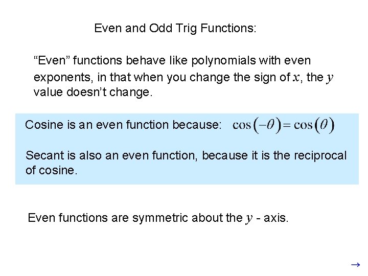
Even and Odd Trig Functions: “Even” functions behave like polynomials with even exponents, in that when you change the sign of x, the y value doesn’t change. Cosine is an even function because: Secant is also an even function, because it is the reciprocal of cosine. Even functions are symmetric about the y - axis.

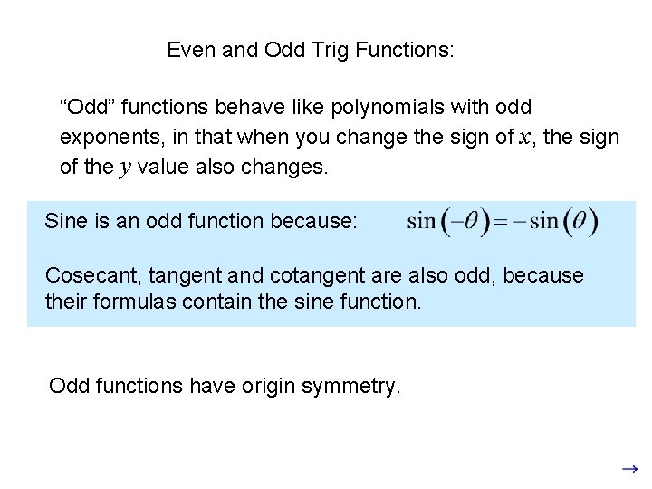
Even and Odd Trig Functions: “Odd” functions behave like polynomials with odd exponents, in that when you change the sign of x, the sign of the y value also changes. Sine is an odd function because: Cosecant, tangent and cotangent are also odd, because their formulas contain the sine function. Odd functions have origin symmetry.

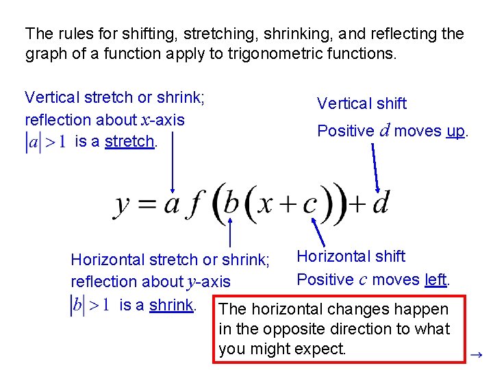
The rules for shifting, stretching, shrinking, and reflecting the graph of a function apply to trigonometric functions. Vertical stretch or shrink; reflection about x-axis is a stretch. Vertical shift Positive d moves up. Horizontal shift Horizontal stretch or shrink; Positive c moves left. reflection about y-axis is a shrink. The horizontal changes happen in the opposite direction to what you might expect.

When we apply these rules to sine and cosine, we use some different terms. is the amplitude. Vertical shift Horizontal shift is the period. B A D C

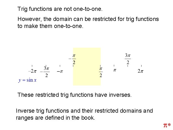
Trig functions are not one-to-one. However, the domain can be restricted for trig functions to make them one-to-one. These restricted trig functions have inverses. Inverse trig functions and their restricted domains and ranges are defined in the book. p*

The sine equation is built into the TI-89 as a sinusoidal regression equation. For practice, we will find the sinusoidal equation for the tuning fork data in the book. To save time, we will use only five points instead of all the data.

Tuning Fork Data Time: Pressure: 2 nd { . 00108. 200 . 00198. 00289. 771 -. 309 . 00108, . 00198, . 00289, . 00379, . 00471 STO 2 nd MATH . 00379. 480 6 Statistics 3 9 alpha Sin. Regressions alpha L 1 , The calculator should return: } 2 nd L 1 alpha . 00471. 581 ENTER L 2 Done ENTER

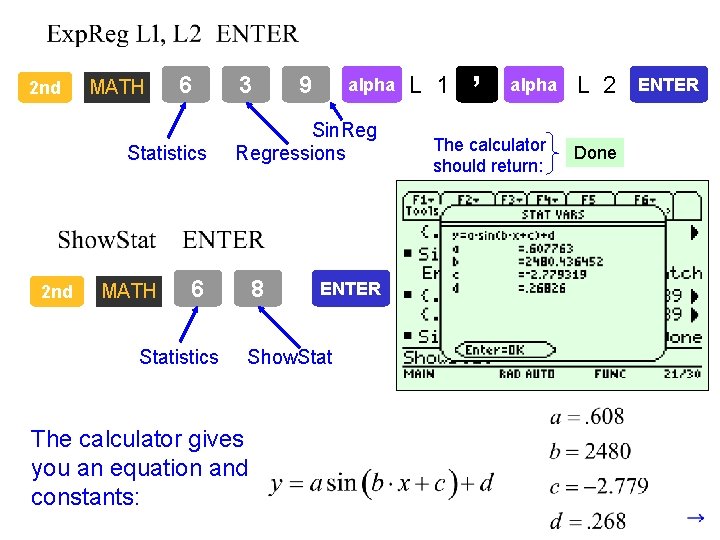
2 nd MATH 6 Statistics 2 nd MATH 3 alpha Sin. Regressions 6 Statistics 9 8 ENTER Show. Stat The calculator gives you an equation and constants: L 1 , alpha The calculator should return: L 2 Done ENTER

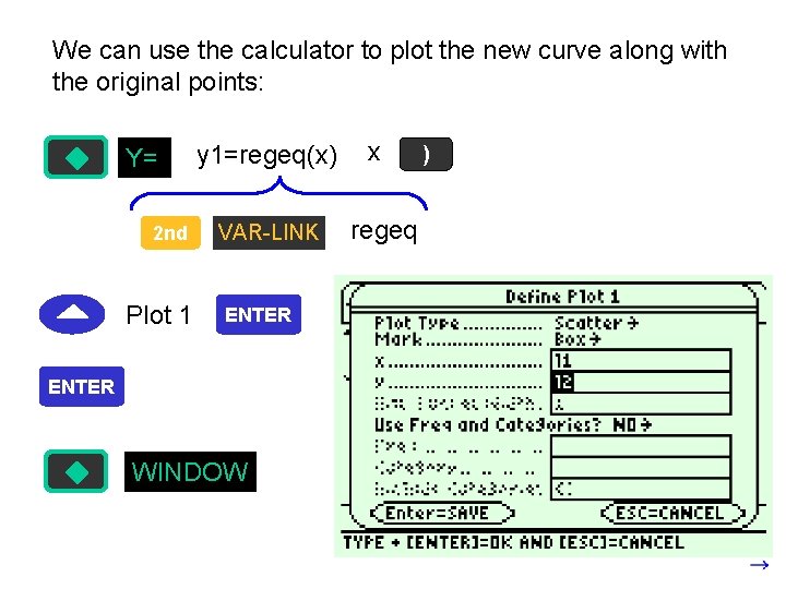
We can use the calculator to plot the new curve along with the original points: Y= 2 nd Plot 1 y 1=regeq(x) VAR-LINK ENTER WINDOW x regeq )

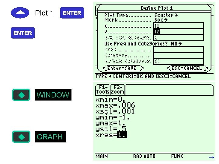
Plot 1 ENTER WINDOW GRAPH

WINDOW GRAPH You could use the “trace” function to investigate the pressure at any given time. p