1 4 4 Sequencing Theory for Single Machine

1

4. 4 Sequencing Theory for Single Machine 1. Shortest Processing Time (SPT) § Minimizes the mean flow time § Minimizes waiting time § Minimizes lateness for single-machine sequencing. 2. Earliest Due Date Scheduling § Minimizes the maximum lateness 2

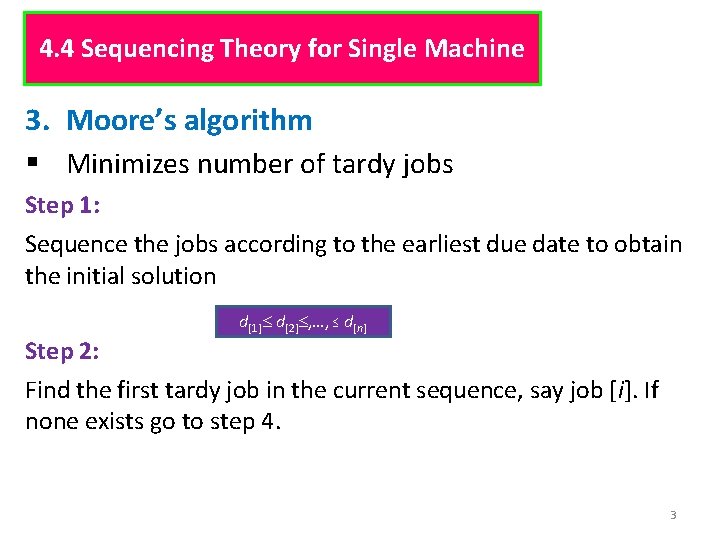
4. 4 Sequencing Theory for Single Machine 3. Moore’s algorithm § Minimizes number of tardy jobs Step 1: Sequence the jobs according to the earliest due date to obtain the initial solution d[1] d[2] , …, d[n] Step 2: Find the first tardy job in the current sequence, say job [i]. If none exists go to step 4. 3

4. 4 Sequencing Theory for Single Machine Step 3: Consider jobs [1], [2], …, [i]. Reject the job with the largest processing time. Return to step 2. Reason: Largest effect on the tardiness of the Job[i] Step 4: Form an optimal sequence by taking the current sequence and appending to it the rejected jobs. The job appended to the current sequence scheduled in any order. Reason: Consider number of tardiness jobs rather than tardiness 4

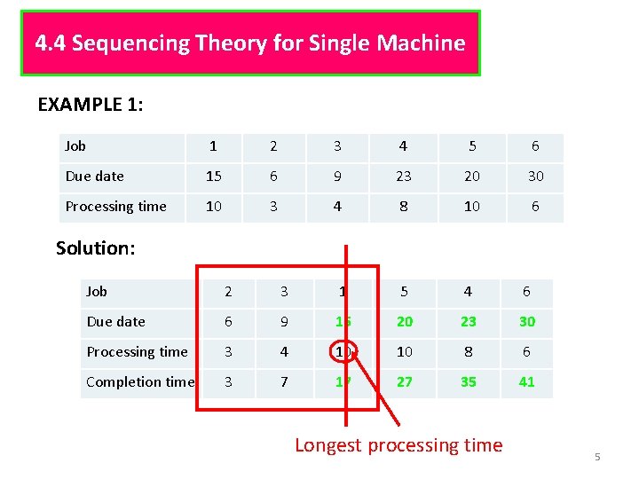
4. 4 Sequencing Theory for Single Machine EXAMPLE 1: Job 1 2 3 4 5 6 Due date 15 6 9 23 20 30 Processing time 10 3 4 8 10 6 Solution: Job 2 3 1 5 4 6 Due date 6 9 15 20 23 30 Processing time 3 4 10 10 8 6 Completion time 3 7 17 27 35 41 Longest processing time 5

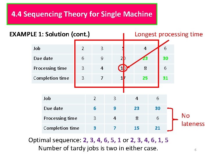
4. 4 Sequencing Theory for Single Machine EXAMPLE 1: Solution (cont. ) Longest processing time Job 2 3 5 4 6 Due date 6 9 20 23 30 Processing time 3 4 10 8 6 Completion time 3 7 17 25 31 Job 2 3 4 6 Due date 6 9 23 30 Processing time 3 4 8 6 Completion time 3 7 15 21 Optimal sequence: 2, 3, 4, 6, 5, 1 or 2, 3, 4, 6, 1, 5 Number of tardy jobs is two in either case. No lateness 6

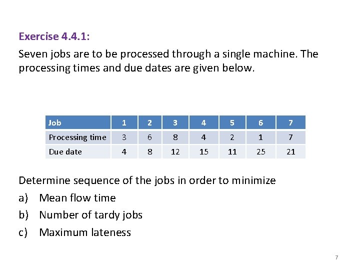
Exercise 4. 4. 1: Seven jobs are to be processed through a single machine. The processing times and due dates are given below. Job 1 2 3 4 5 6 7 Processing time 3 6 8 4 2 1 7 Due date 4 8 12 15 11 25 21 Determine sequence of the jobs in order to minimize a) Mean flow time b) Number of tardy jobs c) Maximum lateness 7

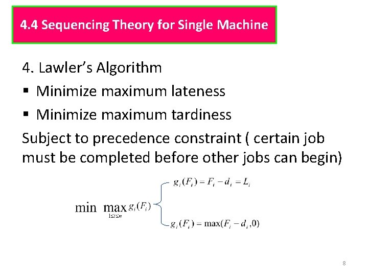
4. 4 Sequencing Theory for Single Machine 4. Lawler’s Algorithm § Minimize maximum lateness § Minimize maximum tardiness Subject to precedence constraint ( certain job must be completed before other jobs can begin) 8

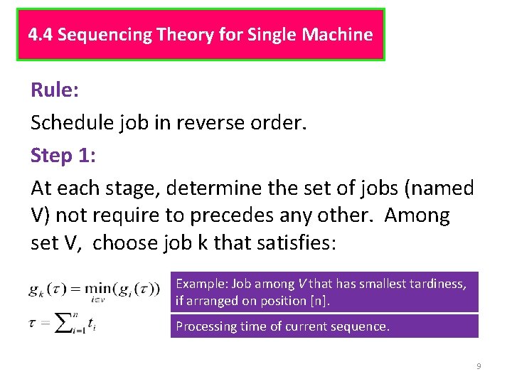
4. 4 Sequencing Theory for Single Machine Rule: Schedule job in reverse order. Step 1: At each stage, determine the set of jobs (named V) not require to precedes any other. Among set V, choose job k that satisfies: Example: Job among V that has smallest tardiness, if arranged on position [n]. Processing time of current sequence. 9

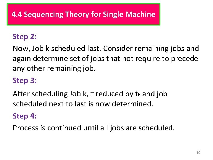
4. 4 Sequencing Theory for Single Machine Step 2: Now, Job k scheduled last. Consider remaining jobs and again determine set of jobs that not require to precede any other remaining job. Step 3: After scheduling Job k, τ reduced by tk and job scheduled next to last is now determined. Step 4: Process is continued until all jobs are scheduled. 10

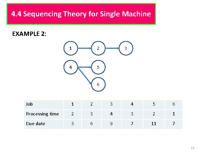
4. 4 Sequencing Theory for Single Machine EXAMPLE 2: 1 2 4 5 3 6 Job 1 2 3 4 5 6 Processing time 2 3 4 3 2 1 Due date 3 6 9 7 11

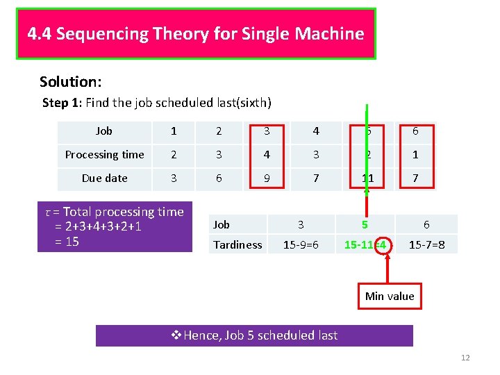
4. 4 Sequencing Theory for Single Machine Solution: Step 1: Find the job scheduled last(sixth) Job 1 2 3 4 5 6 Processing time 2 3 4 3 2 1 Due date 3 6 9 7 11 7 τ = Total processing time = 2+3+4+3+2+1 = 15 Job Tardiness 3 5 6 15 -9=6 15 -11=4 15 -7=8 Min value v. Hence, Job 5 scheduled last 12

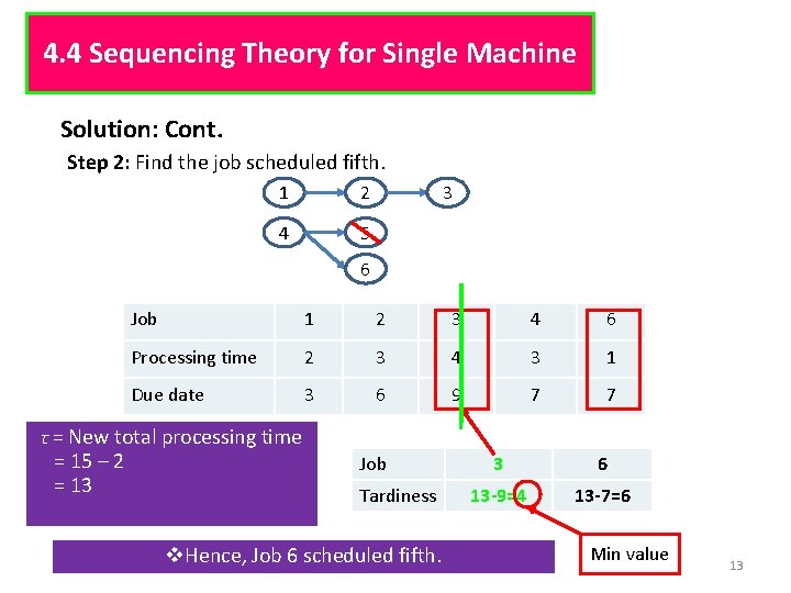
4. 4 Sequencing Theory for Single Machine Solution: Cont. Step 2: Find the job scheduled fifth. 1 2 4 5 3 6 Job 1 2 3 4 6 Processing time 2 3 4 3 1 Due date 3 6 9 7 7 τ = New total processing time = 15 – 2 = 13 Job Tardiness v. Hence, Job 6 scheduled fifth. 3 6 13 -9=4 13 -7=6 Min value 13

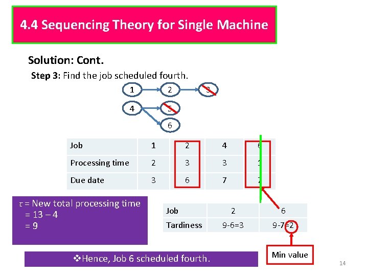
4. 4 Sequencing Theory for Single Machine Solution: Cont. Step 3: Find the job scheduled fourth. 1 2 4 5 3 6 Job 1 2 4 6 Processing time 2 3 3 1 Due date 3 6 7 7 τ = New total processing time = 13 – 4 = 9 Job Tardiness v. Hence, Job 6 scheduled fourth. 2 6 9 -6=3 9 -7=2 Min value 14

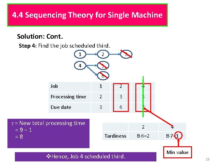
4. 4 Sequencing Theory for Single Machine Solution: Cont. Step 4: Find the job scheduled third. 1 2 4 5 3 6 Job 1 2 4 Processing time 2 3 3 Due date 3 6 7 τ = New total processing time = 9 – 1 = 8 Tardiness v. Hence, Job 4 scheduled third. 2 4 8 -6=2 8 -7=1 Min value 15

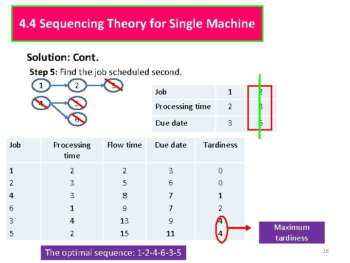
4. 4 Sequencing Theory for Single Machine Solution: Cont. Step 5: Find the job scheduled second. Job 1 2 4 6 3 5 1 2 4 3 Job 1 2 5 Processing time 2 3 6 Due date 3 6 Processing time Flow time Due date Tardiness 2 3 3 1 4 2 2 5 8 9 13 15 3 6 7 7 9 11 0 0 1 2 4 4 The optimal sequence: 1 -2 -4 -6 -3 -5 Maximum tardiness 16

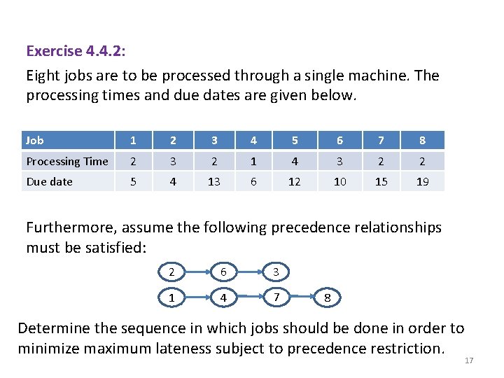
Exercise 4. 4. 2: Eight jobs are to be processed through a single machine. The processing times and due dates are given below. Job 1 2 3 4 5 6 7 8 Processing Time 2 3 2 1 4 3 2 2 Due date 5 4 13 6 12 10 15 19 Furthermore, assume the following precedence relationships must be satisfied: 2 6 3 1 4 7 8 Determine the sequence in which jobs should be done in order to minimize maximum lateness subject to precedence restriction. 17

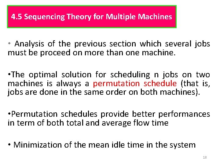
4. 5 Sequencing Theory for Multiple Machines • Analysis of the previous section which several jobs must be proceed on more than one machine. • The optimal solution for scheduling n jobs on two machines is always a permutation schedule (that is, jobs are done in the same order on both machines). • Permutation schedules provide better performances in term of both total and average flow time • Minimization of the mean idle time in the system 18

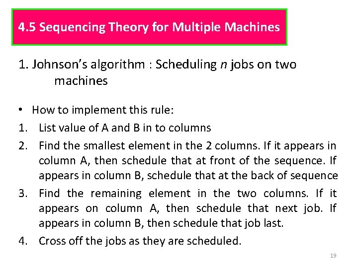
4. 5 Sequencing Theory for Multiple Machines 1. Johnson’s algorithm : Scheduling n jobs on two machines • How to implement this rule: 1. List value of A and B in to columns 2. Find the smallest element in the 2 columns. If it appears in column A, then schedule that at front of the sequence. If appears in column B, schedule that at the back of sequence 3. Find the remaining element in the two columns. If it appears on column A, then schedule that next job. If appears in column B, then schedule that job last. 4. Cross off the jobs as they are scheduled. 19

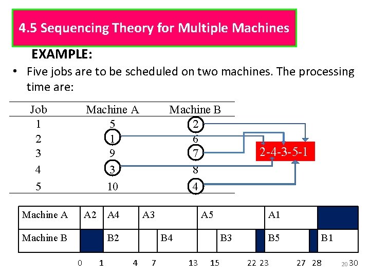
4. 5 Sequencing Theory for Multiple Machines EXAMPLE: • Five jobs are to be scheduled on two machines. The processing time are: Job 1 2 3 4 5 Machine A 5 1 9 3 10 Machine A A 2 A 4 Machine B 2 6 7 8 4 A 3 B 2 0 1 A 5 B 4 4 7 A 1 B 3 13 15 2 -4 -3 -5 -1 B 5 22 23 B 1 27 28 20 30

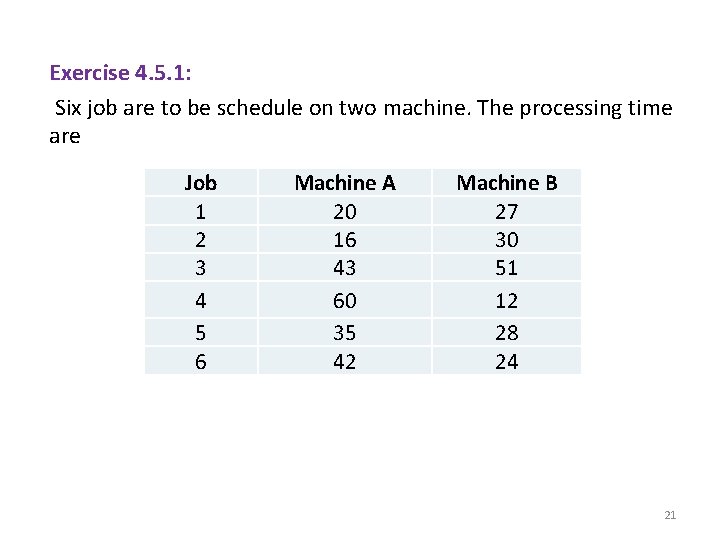
Exercise 4. 5. 1: Six job are to be schedule on two machine. The processing time are Job 1 2 3 4 5 6 Machine A 20 16 43 60 35 42 Machine B 27 30 51 12 28 24 21

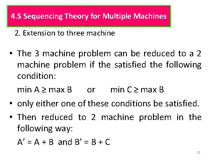
4. 5 Sequencing Theory for Multiple Machines 2. Extension to three machine • The 3 machine problem can be reduced to a 2 machine problem if the satisfied the following condition: min A ≥ max B or min C ≥ max B • only either one of these conditions be satisfied. • Then reduced to 2 machine problem in the following way: A’ = A + B and B’ = B + C 22

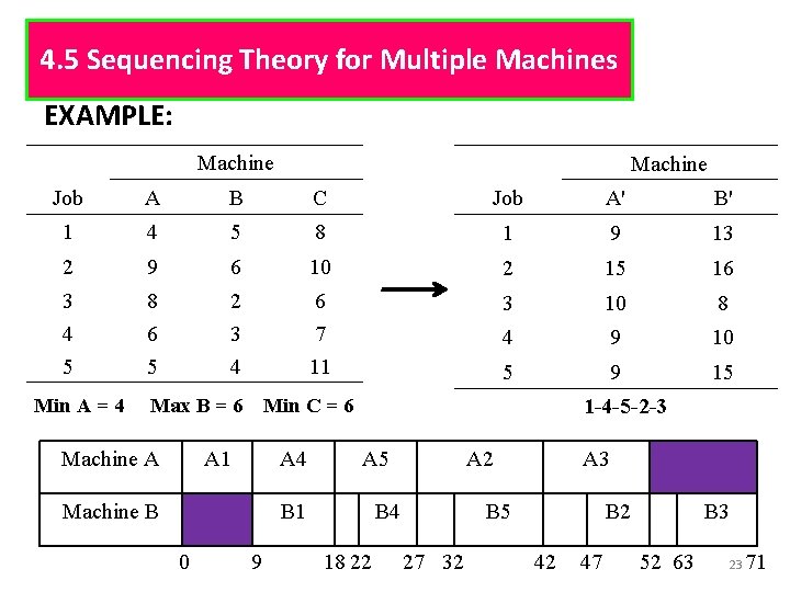
4. 5 Sequencing Theory for Multiple Machines EXAMPLE: Machine Job A B C Job A' B' 1 4 5 8 1 9 13 2 9 6 10 2 15 16 3 4 5 8 6 5 2 3 4 6 7 11 3 10 8 4 9 10 5 9 15 Min A = 4 Max B = 6 Machine A Min C = 6 A 1 A 4 Machine B 1 -4 -5 -2 -3 A 5 B 1 0 9 A 2 B 4 18 22 A 3 B 5 27 32 B 2 42 47 B 3 52 63 23 71

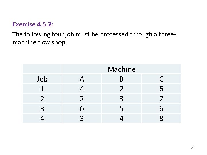
Exercise 4. 5. 2: The following four job must be processed through a threemachine flow shop Job 1 2 3 4 A 4 2 6 3 Machine B 2 3 5 4 C 6 7 6 8 24

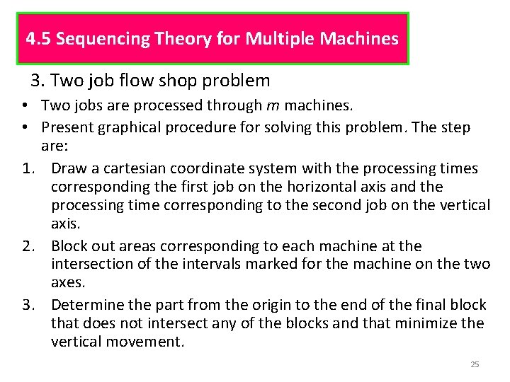
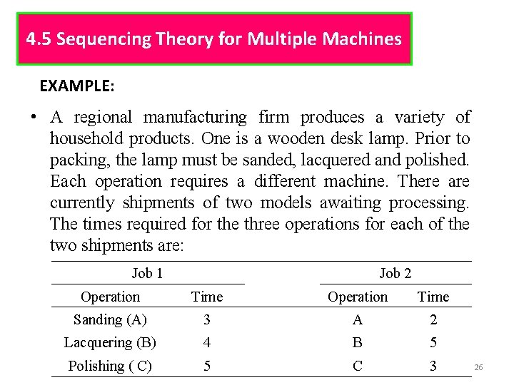
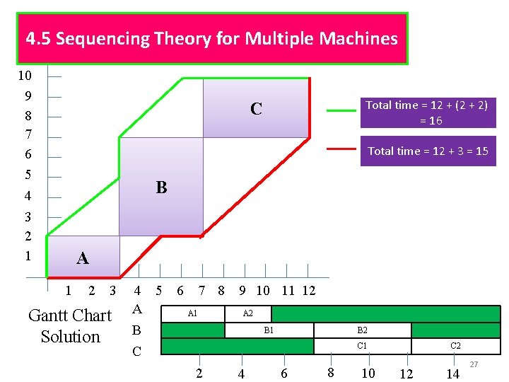
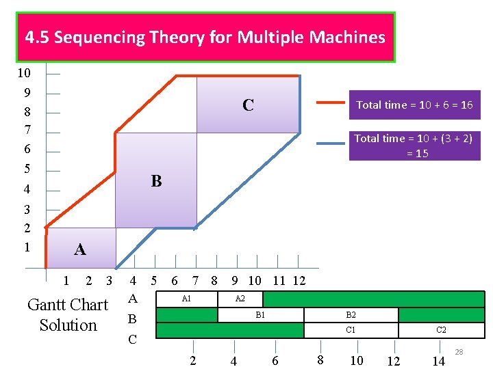
4. 5 Sequencing Theory for Multiple Machines 3. Two job flow shop problem • Two jobs are processed through m machines. • Present graphical procedure for solving this problem. The step are: 1. Draw a cartesian coordinate system with the processing times corresponding the first job on the horizontal axis and the processing time corresponding to the second job on the vertical axis. 2. Block out areas corresponding to each machine at the intersection of the intervals marked for the machine on the two axes. 3. Determine the part from the origin to the end of the final block that does not intersect any of the blocks and that minimize the vertical movement. 25

4. 5 Sequencing Theory for Multiple Machines EXAMPLE: • A regional manufacturing firm produces a variety of household products. One is a wooden desk lamp. Prior to packing, the lamp must be sanded, lacquered and polished. Each operation requires a different machine. There are currently shipments of two models awaiting processing. The times required for the three operations for each of the two shipments are: Job 1 Operation Time Sanding (A) Job 2 Operation Time 3 A 2 Lacquering (B) 4 B 5 Polishing ( C) 5 C 3 26

4. 5 Sequencing Theory for Multiple Machines 10 9 8 7 6 5 Total time = 12 + (2 + 2) = 16 C Total time = 12 + 3 = 15 B 4 3 2 1 A 1 2 3 Gantt Chart Solution 4 5 A B C 6 7 8 A 1 9 10 11 12 A 2 B 1 B 2 C 1 2 4 6 8 10 C 2 12 14 27

4. 5 Sequencing Theory for Multiple Machines 10 9 8 7 6 5 C Total time = 10 + 6 = 16 Total time = 10 + (3 + 2) = 15 B 4 3 2 1 A 1 2 3 Gantt Chart Solution 4 5 A B C 6 7 8 A 1 9 10 11 12 A 2 B 1 B 2 C 1 2 4 6 8 10 C 2 12 14 28

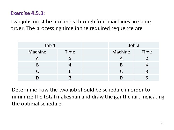
Exercise 4. 5. 3: Two jobs must be proceeds through four machines in same order. The processing time in the required sequence are Job 1 Machine A B C D Time 5 4 6 3 Job 2 Machine Time A 2 B 4 C 3 D 5 Determine how the two job should be schedule in order to minimize the total makespan and draw the gantt chart indicating the optimal schedule. 29

4. 6 ASSEMBLY LINE BALANCING Line Balancing Line balancing: the process of assigning tasks to workstations in such a way that the workstations have approximately equal time requirements. Cycle Time Cycle time: maximum time allowed at each workstation to complete its set of tasks on a unit. amount of time allotted to each workstation determined in advance, based on the desired rate of production of assembly line. Maximum cycle time = summation of the task times. Minimum cycle time = the longest task times. 30

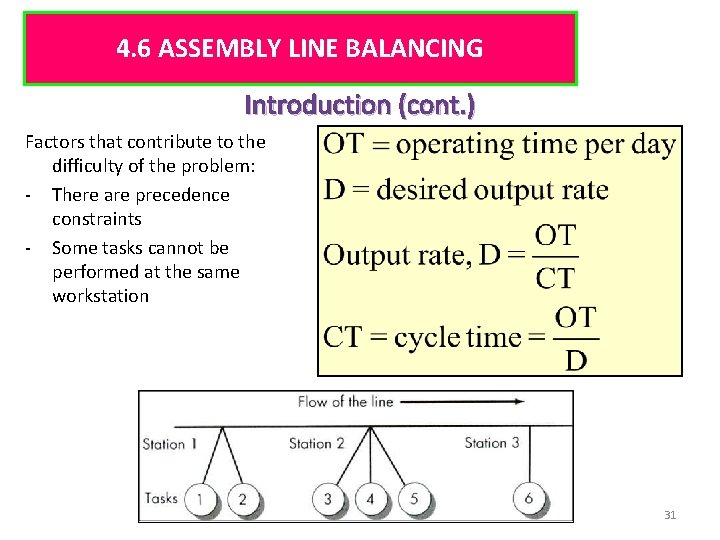
4. 6 ASSEMBLY LINE BALANCING Introduction (cont. ) Factors that contribute to the difficulty of the problem: - There are precedence constraints - Some tasks cannot be performed at the same workstation 31

4. 6 ASSEMBLY LINE BALANCING Line Balancing Rules Some Heuristic (intuitive) Rules: • Assign tasks in order of most following tasks. – Count the number of tasks that follow • Assign tasks in order of greatest positional weight. – Positional weight is the sum of each task’s time and the times of all following tasks. 32

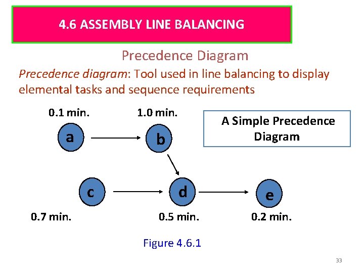
4. 6 ASSEMBLY LINE BALANCING Precedence Diagram Precedence diagram: Tool used in line balancing to display elemental tasks and sequence requirements 0. 1 min. 1. 0 min. a b c 0. 7 min. A Simple Precedence Diagram d 0. 5 min. e 0. 2 min. Figure 4. 6. 1 33

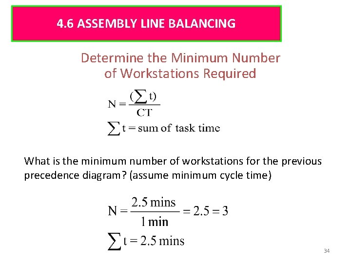
4. 6 ASSEMBLY LINE BALANCING Determine the Minimum Number of Workstations Required What is the minimum number of workstations for the previous precedence diagram? (assume minimum cycle time) 34

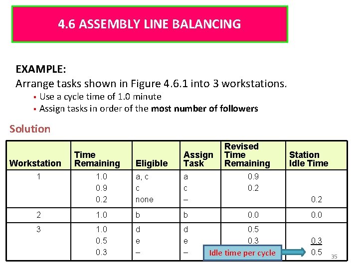
4. 6 ASSEMBLY LINE BALANCING EXAMPLE: Arrange tasks shown in Figure 4. 6. 1 into 3 workstations. § Use a cycle time of 1. 0 minute § Assign tasks in order of the most number of followers Solution Eligible Assign Task 1. 0 0. 9 0. 2 a, c c none a c – 0. 9 0. 2 2 1. 0 b b 0. 0 3 1. 0 0. 5 0. 3 d e – 0. 5 0. 3 Workstation 1 Time Remaining Revised Time Remaining Station Idle Time 0. 2 Idle time per cycle 0. 0 0. 3 0. 5 35

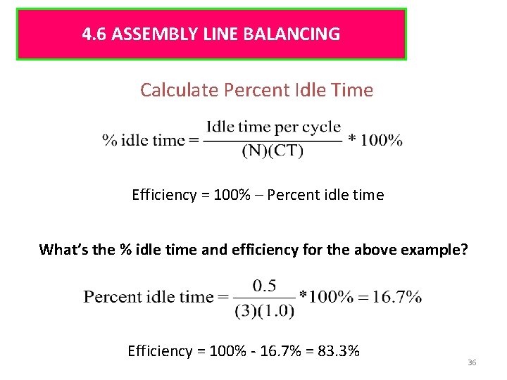
4. 6 ASSEMBLY LINE BALANCING Calculate Percent Idle Time Efficiency = 100% – Percent idle time What’s the % idle time and efficiency for the above example? Efficiency = 100% - 16. 7% = 83. 3% 36

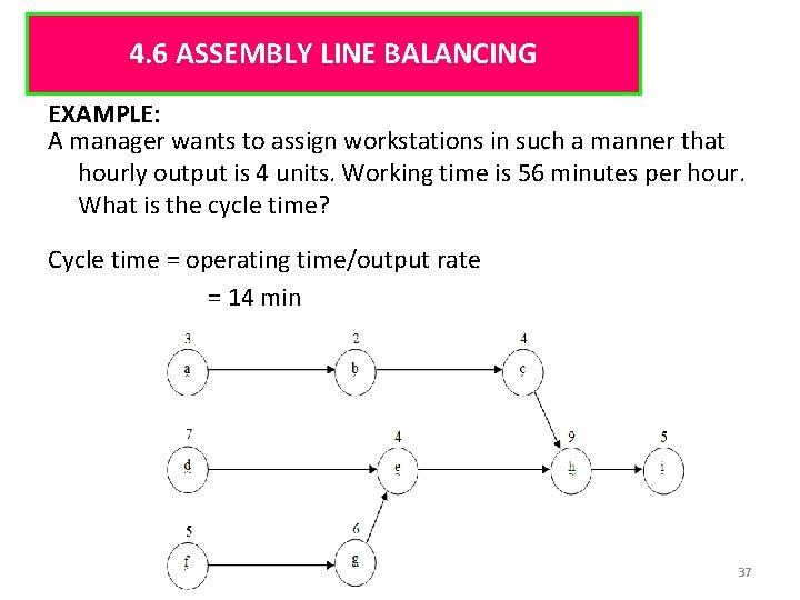
4. 6 ASSEMBLY LINE BALANCING EXAMPLE: A manager wants to assign workstations in such a manner that hourly output is 4 units. Working time is 56 minutes per hour. What is the cycle time? Cycle time = operating time/output rate = 14 min 37

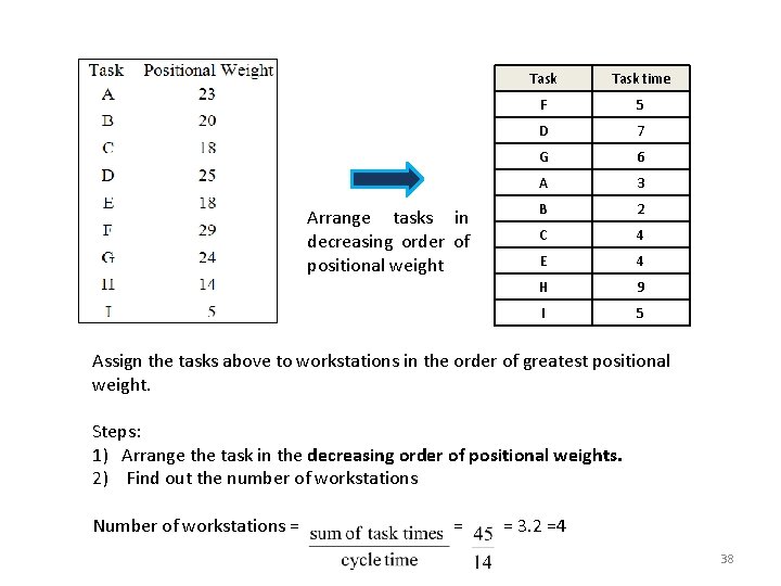
Arrange tasks in decreasing order of positional weight Task time F 5 D 7 G 6 A 3 B 2 C 4 E 4 H 9 I 5 Assign the tasks above to workstations in the order of greatest positional weight. Steps: 1) Arrange the task in the decreasing order of positional weights. 2) Find out the number of workstations Number of workstations = = 3. 2 =4 38

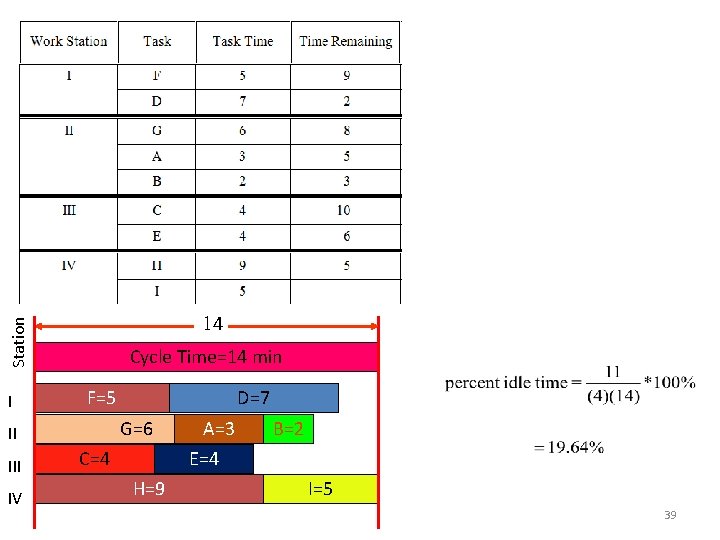
Station I II IV 14 Cycle Time=14 min F=5 G=6 C=4 H=9 D=7 A=3 E=4 B=2 I=5 39

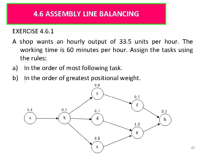
4. 6 ASSEMBLY LINE BALANCING EXERCISE 4. 6. 1 A shop wants an hourly output of 33. 5 units per hour. The working time is 60 minutes per hour. Assign the tasks using the rules: a) In the order of most following task. b) In the order of greatest positional weight. 40

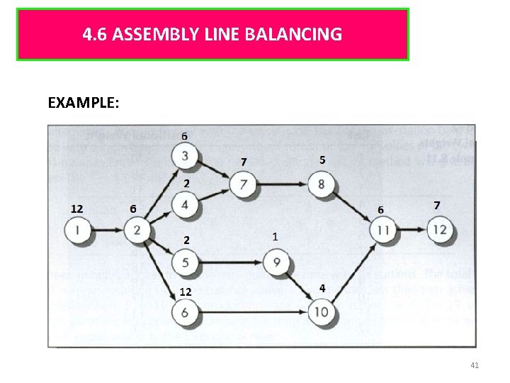
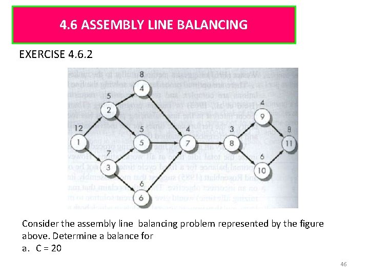
4. 6 ASSEMBLY LINE BALANCING EXAMPLE: 41

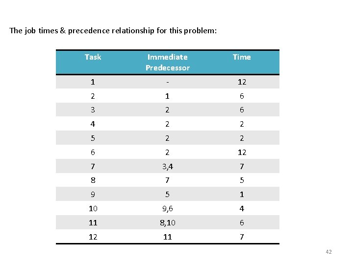
The job times & precedence relationship for this problem: Task Immediate Predecessor Time 1 - 12 2 1 6 3 2 6 4 2 2 5 2 2 6 2 12 7 3, 4 7 8 7 5 9 5 1 10 9, 6 4 11 8, 10 6 12 11 7 42

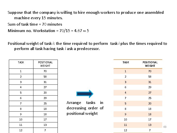
Suppose that the company is willing to hire enough workers to produce one assembled machine every 15 minutes. Sum of task time = 70 minutes Minimum no. Workstation = 70/15 = 4. 67 5 Positional weight of task i: the time required to perform task i plus the times required to perform all task having task i ask a predecessor. TASK POSITIONAL WEIGHT 1 70 2 58 3 31 4 27 6 29 5 20 4 27 6 29 7 25 5 20 8 18 9 18 10 17 11 13 12 7 Arrange tasks in decreasing order of positional weight 43

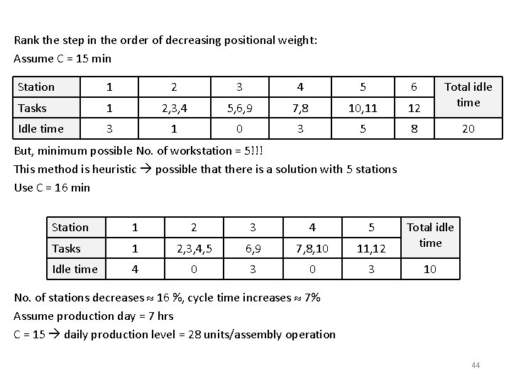
Rank the step in the order of decreasing positional weight: Assume C = 15 min Station 1 2 3 4 5 6 Tasks 1 2, 3, 4 5, 6, 9 7, 8 10, 11 12 Total idle time Idle time 3 1 0 3 5 8 20 But, minimum possible No. of workstation = 5!!! This method is heuristic possible that there is a solution with 5 stations Use C = 16 min Station 1 2 3 4 5 Tasks 1 2, 3, 4, 5 6, 9 7, 8, 10 11, 12 Total idle time Idle time 4 0 3 10 No. of stations decreases 16 %, cycle time increases 7% Assume production day = 7 hrs C = 15 daily production level = 28 units/assembly operation 44

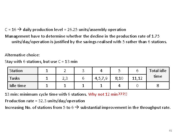
C = 16 daily production level = 26. 25 units/assembly operation Management have to determine whether the decline in the production rate of 1. 75 units/day/operation is justified by the savings realised with 5 rather than 6 stations. Alternative choice: Stay with 6 stations, but use C = 13 min Station 1 2 3 4 5 6 Tasks 1 2, 3 6 4, 5, 7, 9 8, 10 11, 12 Total idle time Idle time 1 1 4 0 8 13 min: minimum cycle time with 6 stations. Why not 12 min? ? ? !! Production rate = 32. 3 units/day/operation Increasing No. of stations from 5 to 6 substantial improvement in the throughput rate. 45

4. 6 ASSEMBLY LINE BALANCING EXERCISE 4. 6. 2 Consider the assembly line balancing problem represented by the figure above. Determine a balance for a. C = 20 46

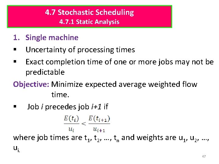
4. 7 Stochastic Scheduling 4. 7. 1 Static Analysis 1. Single machine § Uncertainty of processing times § Exact completion time of one or more jobs may not be predictable Objective: Minimize expected average weighted flow time. § Job i precedes job i+1 if where job times are t 1, t 2, …, tn and weights are u 1, u 2, …, ui. 47

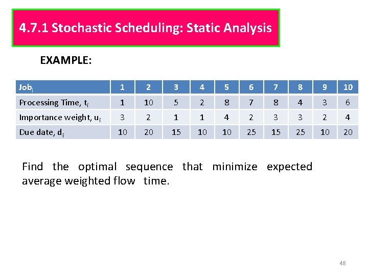
4. 7. 1 Stochastic Scheduling: Static Analysis EXAMPLE: Jobi 1 2 3 4 5 6 7 8 9 10 Processing Time, ti 1 10 5 2 8 7 8 4 3 6 Importance weight, ui 3 2 1 1 4 2 3 3 2 4 Due date, di 10 20 15 10 10 25 15 25 10 20 Find the optimal sequence that minimize expected average weighted flow time. 48

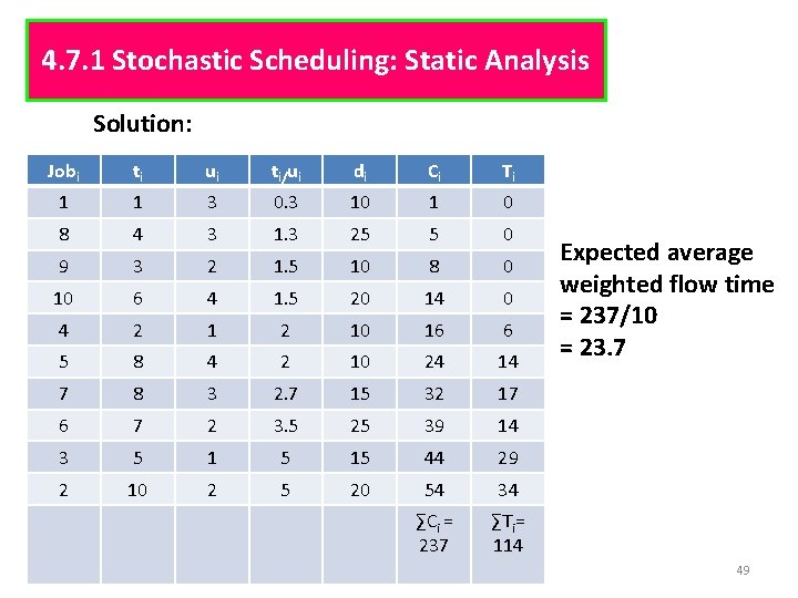
4. 7. 1 Stochastic Scheduling: Static Analysis Solution: Jobi ti ui ti/ui di Ci Ti 1 1 3 0. 3 10 1 0 8 4 3 1. 3 25 5 0 9 3 2 1. 5 10 8 0 10 6 4 1. 5 20 14 0 4 2 10 16 6 5 8 4 2 10 24 14 7 8 3 2. 7 15 32 17 6 7 2 3. 5 25 39 14 3 5 15 44 29 2 10 2 5 20 54 34 ∑Ci = 237 ∑Ti= 114 Expected average weighted flow time = 237/10 = 23. 7 49

4. 7. 1 Stochastic Scheduling: Static Analysis 2. Multiple Machine • n jobs are to processed through two identical parallel machines. Each jobs needs to be processed only once on either machine. • The objective is to minimize the expected makespan. • Parallel is different from flow shop problem. • In flow shop, jobs are processed first one machine 1 then on machine 2. • Then the optimal sequence is to schedule the jobs according to LEPT (longest expected processing time first) opposite with the SPT rule 50

4. 7. 2 Stochastic Scheduling: Dynamic Analysis Dynamic: Jobs arrive randomly over time, and decisions must be made on an ongoing basis as how to schedule those jobs. §When jobs arrive shop dynamically over time, queuing theory provides a means of analyzing the results. § Standard M/M/1 queue applies to case of purely random arrivals to single machine with random processing times. 51

4. 7. 2 Stochastic Scheduling: Dynamic Analysis Selection independent of job processing times § Same mean flow times, but differ variance flow times Selection dependent of job processing times § Job times realized when job joins the queue rather than when job enters service § SPT results lowest expected flow time. 52

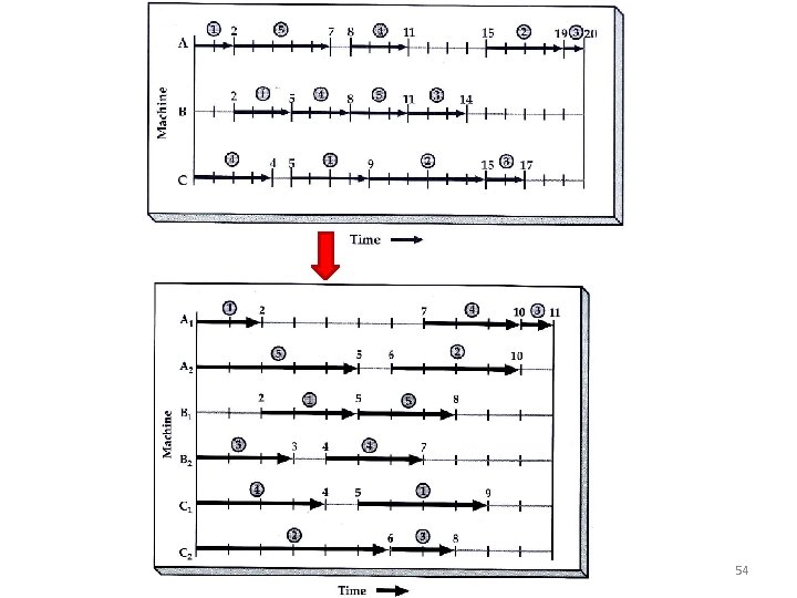
4. 8 ADVANCED TOPIC FOR OPERATIONS SCHEDULING 4. 8. 1 FINITE CAPACITY PLANNING (FCS) FCS - jobs are being scheduled through a number of work centers, each with one or more machines. • jobs can pass each other or change their order as they are processed, depending on their priority. • a job can be split into two or more parts if this will facilitate scheduling Advantage: -The addition of capacity improves completion dates of jobs & reduces waiting times. Bottleneck: a work centre whose capacity is less than the demand placed on it & less than the capacities of all other resources. 53

54

4. 8. 2 BATCH SCHEDULING Batch operation: Job shop “shop”, “job”, “work center” Job “customer”, “patient”, “client”, “paperwork” Work centre “room”, “office”, “facility”, “skill specialty” In a job shop, batch corresponds to what customer orders – can include one or several parts or items. Each part or job is scheduled through the various machines & work centres according to the equipment & labour needed to process the job. 55

Batch scheduling: • each batch flowing through a batch process typically moves along with many starts & stops, not smoothly – due to layout of batch process jobs or customers wait in line as each batch is transferred from one work centre to the next. • batch scheduling problem: network or queues. • Jobs or customers spend most of their time waiting in line – amount of time waiting varies with the load of the process 56

Thank You ^^ 57