1 3 Linear Functions and Mathematical Models Mathematics

1. 3 Linear Functions and Mathematical Models • Mathematics can be used to solve real-world problems. • Regardless of the field from which the real-world problem is drawn, the problem is analyzed using a process called mathematical modeling. The relation between two quantities is conveniently described in mathematics by using the concept of a function. Copyright © 2006 Brooks/Cole, a division of Thomson Learning, Inc.

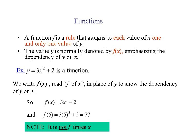
Functions • A function f is a rule that assigns to each value of x one and only one value of y. • The value y is normally denoted by f(x), emphasizing the dependency of y on x. We write f (x) , read “f of x”, in place of y to show the dependency of y on x. So and NOTE: It is not f times x

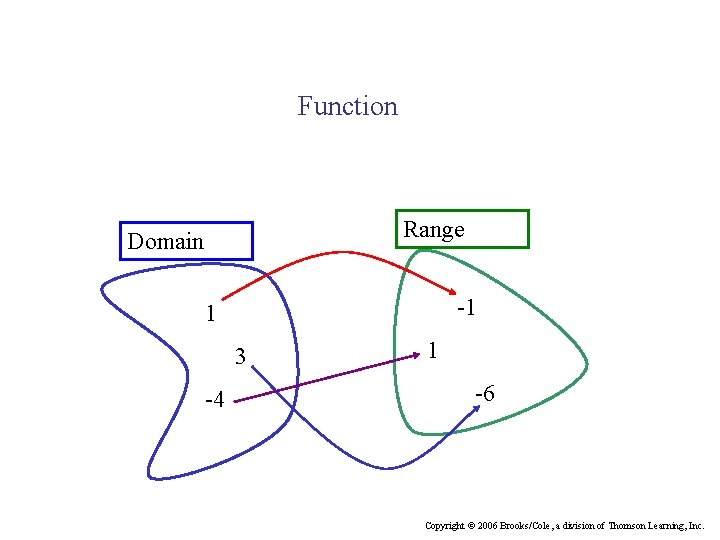
Function Range Domain -1 1 3 -4 1 -6 Copyright © 2006 Brooks/Cole, a division of Thomson Learning, Inc.

Domain and Range Suppose we are given the function y = f(x). • The variable x is referred to as the independent variable, and the variable y is called the dependent variable. • The set of all the possible values of x is called the domain of the function f. • The set of all the values of f(x) resulting from all the possible values of x in its domain is called the range of f. • The output f(x) associated with an input x is unique: – Each x must correspond to one and only one value of f(x).

Linear Function A linear function can be expressed in the form m and b are constants It can be used for • Simple Depreciation • Linear Supply and Demand Functions • Linear Cost, Revenue, and Profit Functions Copyright © 2006 Brooks/Cole, a division of Thomson Learning, Inc.

Simple Depreciation Ex. A computer with original value $2000 is linearly depreciated to a value of $200 after 4 years. Find an equation for the value, V, of the computer at the end of year t. What will be the computer value at the end of the third year? What is the rate of depreciation of the computer? Copyright © 2006 Brooks/Cole, a division of Thomson Learning, Inc.

Solution: Since the depreciation is linear, V is a linear function of t. Equivalently, The graph of the function is a straight line. Observe that V=2000 when t=0, and V=200 when t=4. This tells us that the line passes through the points The slope of the line is given by

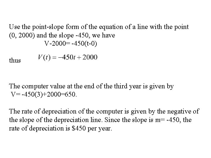
Use the point-slope form of the equation of a line with the point (0, 2000) and the slope -450, we have V-2000= -450(t-0) thus The computer value at the end of the third year is given by V= -450(3)+2000=650. The rate of depreciation of the computer is given by the negative of the slope of the depreciation line. Since the slope is m= -450, the rate of depreciation is $450 per year.

Example: A car purchased for use by the manager of a firm at a price of $24, 000 is to be depreciated using the straight line method over 5 years. What will be the book value of the car at the end of 3 year? (Assume the scrap value is $0. ) Solution: Let V(t) be the value of the car at the end of tth year. When t = 0, V = 24, 000; when t = 5, V = 0 Then b = 24, 000

Then the equation is V=-4, 800 t+24, 000 When t=3, V=-4, 800(3)+24, 000=9, 600 So the book value of the car at the end of 3 year is $9, 600.

Cost, Revenue, and Profit Functions Let x denote the number of nits of a product manufactured or sold. • Then the total cost function is C (x)=Total cost of manufacturing x units of the product • The revenue function is R(x) = Total revenue realized from the sale of x units of the product. • The profit function is P(x)= Total profit realized from manufacturing and selling x units of product.

Suppose a firm has a fixed cost of F dollars, a production cost of c dollars per unit, and a selling price of s dollars per unit. Then the cost function C(x), the revenue function R(x), and the profit function P(x) for the firm are given by C (x) = c x + F R (x) = s x P (x) = R (x) – C (x) = (s - c) x- F

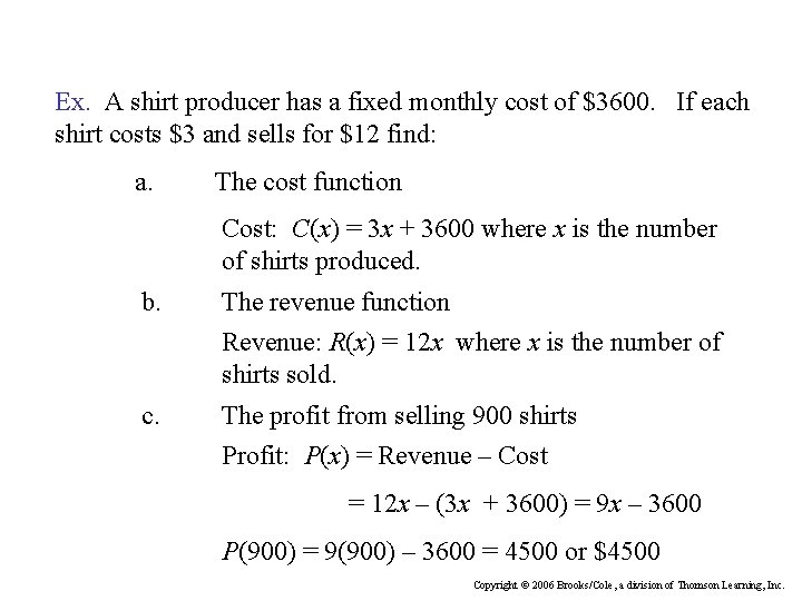
Ex. A shirt producer has a fixed monthly cost of $3600. If each shirt costs $3 and sells for $12 find: a. The cost function Cost: C(x) = 3 x + 3600 where x is the number of shirts produced. b. The revenue function Revenue: R(x) = 12 x where x is the number of shirts sold. c. The profit from selling 900 shirts Profit: P(x) = Revenue – Cost = 12 x – (3 x + 3600) = 9 x – 3600 P(900) = 9(900) – 3600 = 4500 or $4500 Copyright © 2006 Brooks/Cole, a division of Thomson Learning, Inc.

Linear Demand Supply Curves A demand equation expresses the relation between the unit price and the quantity demanded. The corresponding graph of the demand equation is called a demand curve. A demand function, defined by p=f(x), where p measures the unit price and x measures the number of units of commodity, is generally characterized as a decreasing function of x; that is, p=f(x) decreases as x increases.

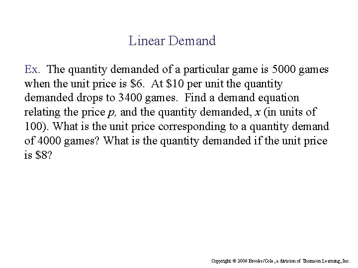
Linear Demand Ex. The quantity demanded of a particular game is 5000 games when the unit price is $6. At $10 per unit the quantity demanded drops to 3400 games. Find a demand equation relating the price p, and the quantity demanded, x (in units of 100). What is the unit price corresponding to a quantity demand of 4000 games? What is the quantity demanded if the unit price is $8? Copyright © 2006 Brooks/Cole, a division of Thomson Learning, Inc.

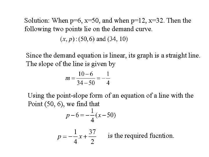
Solution: When p=6, x=50, and when p=12, x=32. Then the following two points lie on the demand curve. Since the demand equation is linear, its graph is a straight line. The slope of the line is given by Using the point-slope form of an equation of a line with the Point (50, 6), we find that is the required fucntion.

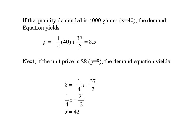
If the quantity demanded is 4000 games (x=40), the demand Equation yields Next, if the unit price is $8 (p=8), the demand equation yields

Supply Function An equation that expresses the relationship between the unit price And the quantity supplied is called a supply equation, and the Corresponding graph is called a supply curve. A supply function, defined by p = f (x), is generally characterized by Increasing function of x; that is, p = f (x) increases as x increases.