1 1957 2 U Fano Phys Rev 124

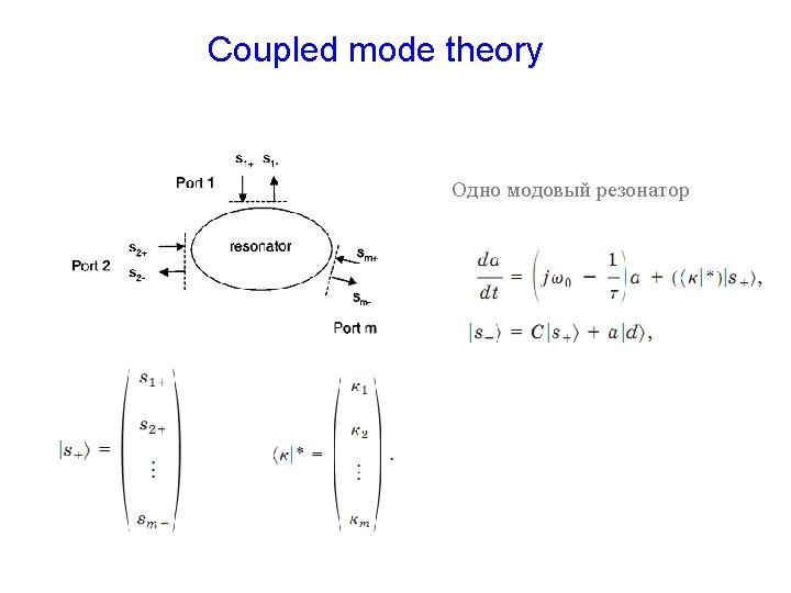
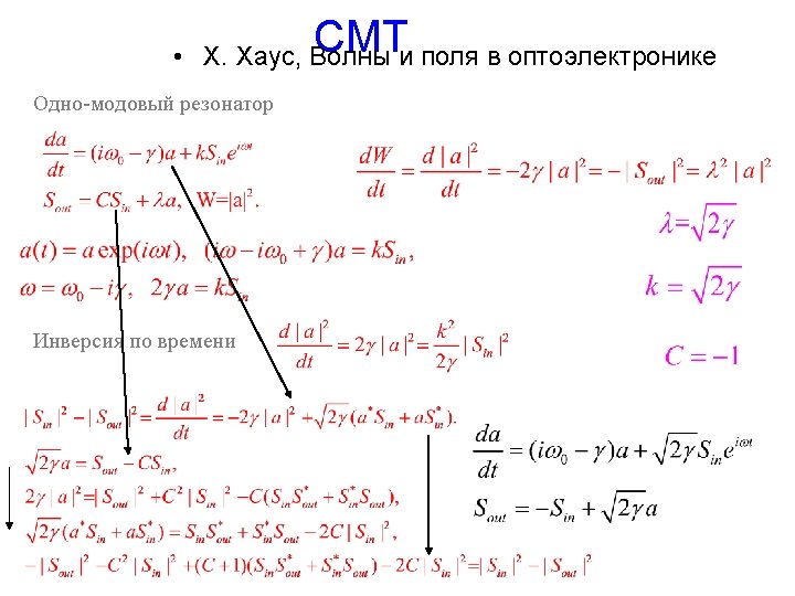
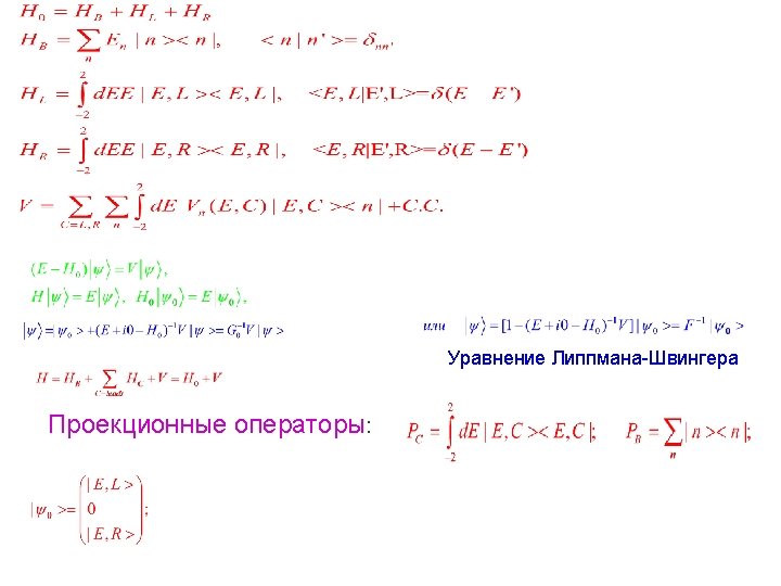
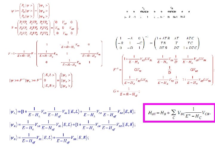
Подход эффективного гамильтониана 1. М. С. Лифшиц, ЖЭТФ (1957). 2. U. Fano, Phys. Rev. 124, 1866 (1961). 3. H. Feshbach, , Ann. Phys. (New York) 5 (1958) 357; 19 (1962) 287. 4. C. Mahaux, H. A. Weidenmuller, (Shell-Model Approach to Nuclear Reactions), North-Holland, Amsterdam, 1969. 5. I. Rotter, Rep. Prog. Phys. , 54, 635 (1991). 6. S. Datta, (Electronic transport in mesoscopic systems) (1995). 7. S. Albeverio, et al J. Math. Phys. 37, 4888 (1996). 8. Y. V. Fyodorov and H. -J. Sommers, J. Math. Phys. 38, 1918 (1997) 9. F. Dittes, Phys. Rep. (2002). 10. Sadreev and I. Rotter, J. Phys. A (2003). 11. J. Okolowicz, M. Ploszajczak, and I. Rotter, Phys. Rep. 374, 271(2003). 12. D. V. Savin, V. V. Sokolov V. V. , and H. -J. Sommers, PRE (2003). 13. Sadreev, J. Phys. A (2012). • Coupled mode theory (оптика) H. A. Haus, (Waves and Fields in Optoelectronics) (1984). C. Manolatou, et al, IEEE J. Quantum Electron. (1999). S. Fan, et al, J. Opt. Soc. Am. A 20, 569 (2003). S. Fan, et al, Phys. Rev. B 59, 15882 (1999). W. Suh, et al, IEEE J. of Quantum Electronics, 40, 1511 (2004). Bulgakov and Sadreev, Phys. Rev. B 78, 075105 (2008).

Coupled defect mode with propagating over waveguide light Manolatou, et al, IEEE J. Quant. Electronics, (1999)

CMT • Много-модовый резонатор IEEE J. Quantum Electronics, 40, 1511 (2004)

Два порта, две моды %CMT for transmission through resonator with two modes clear all E=-2: 0. 01: 2; D=[sqrt(0. 1) sqrt(0. 25)]; G=0. 5*D'*D; H 0=diag([-0. 25]); H=H 0 -1 i*G; for j=1: length(E) Q=E(j)*diag([1 1])-H; in=[1; 0]; IN=1 i*D'*in; A=QIN; ; A 1(j)=A(1); A 2(j)=A(2); t(: , j)=-in+D*A; end

W is matrix Nx. M where N is the number of eigen states of closed quantum system, M is the number of continuums (channels)

S. Datta, (Electronic transport in mesoscopic systems) (1995).

S-matrix Basis of closed billiard The biorthogonal basis

c H. -W. Lee, Generic Transmission Zeros and In-Phase Resonances in Time-Reversal Symmetric Single Channel Transport, Phys. Rev. Lett. 82, 2358 (1999)

2 d case Limit to continual case

Na=input('input length along transport Na=') Nb=input('input length cross to transport Nb=') Nin=input('input numerical position of the input lead Nin=') Nout=input('input numerical position of the output lead Nout=') NL=length(Nin); NR=length(Nout); v. L=1; v. R=v. L; tb=1; %Leads E=-2. 9: 0. 011: 1; HL=zeros(NL, NL); HL=HL-diag(ones(1, NL-1), 1); HL=HL+HL'; HL=HL-diag(sum(HL), 0); for np=1: NL kpp=acos(-E/2+EL(np, np)/2); kp(np, 1: length(E))=kpp; end HR=HL; %Dot N=Na*Nb; HB=zeros(N, N); HB=HB-diag(ones(1, N-1), 1)-diag(ones(1, N-Na), Na); HB(Na: N-Na, Na+1: Na: N-Na+1)=0; HB=tb*(HB+HB'); %Coupling matrix psi. Bin=psi. B(Nin, : ); psi. Bout=psi. B(Nout, : ); WL=v. L*psi. Bin'*psi. L'; WR=v. R*psi. Bout'*psi. L'; DB=diag(ones(Na*Nb, 1)); for j=1: length(E) g=diag(exp(i*kp(: , j))); gg=diag(sin(real(kp(: , j))). ^0. 5); WW=WL*g*WL'+WR*g*WR'; Heff=diag(EB)-WW; QQ=DB*E(j)-Heff; PP=QQ^(-1); SS=2*i*(WL*gg)'*PP*WR*gg; t(n, j)=SS(1, 1); Matlab calculation

Datta’s site representation

Effective Hamiltonian for time-periodic case For stationary case l

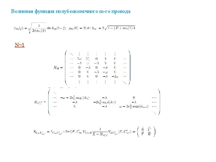
Numerical results N=1 l=0. 75, v. C=0. 25 m=-1, 0, 1 21 quasi energies H. Fukuyama, R. A. Bari, and H. C. Fogedby, PRB (1973). BS, J. Phys. C (1999): Критерий применимости теории возмущений