022812 Photo Stitching Panoramas from Multiple Images Computer

02/28/12 Photo Stitching Panoramas from Multiple Images Computer Vision CS 543 / ECE 549 University of Illinois Derek Hoiem

Homeworks • HW 2 due today – Will try to have it graded by Mar 8 (ECCV deadline on March 5) • HW 3 has been released (due in 2 weeks) • Who designs/grades? – Derek mainly for HW 1, HW 3, HW 5 – Ruiqi mainly for HW 2, HW 4

News

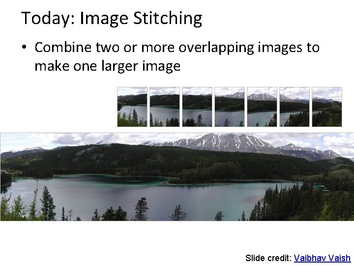
Today: Image Stitching • Combine two or more overlapping images to make one larger image Add example Slide credit: Vaibhav Vaish

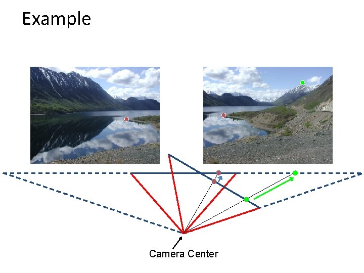
Example Camera Center

Problem set-up • x = K [R t] X • x' = K' [R' t'] X • t=t'=0 . X x x' f f' • x'=Hx where H = K' R' R-1 K-1 • Typically only R and f will change (4 parameters), but, in general, H has 8 parameters

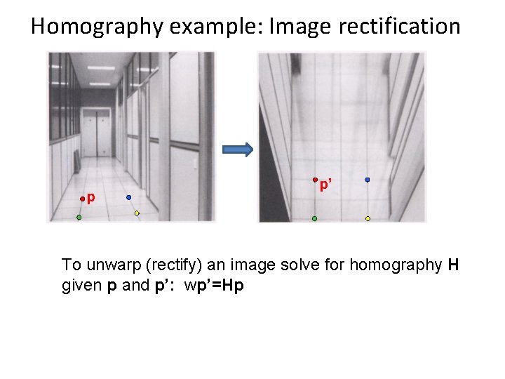
Homography • Definition – General mathematics: homography = projective linear transformation – Vision (most common usage): homography = linear transformation between two image planes • Examples – Project 3 D surface into frontal view – Relate two views that differ only by rotation

Homography example: Image rectification p p’ To unwarp (rectify) an image solve for homography H given p and p’: wp’=Hp

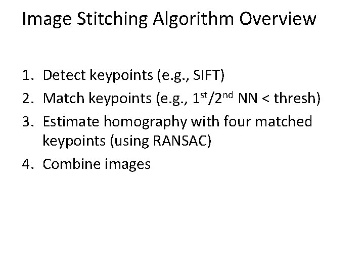
Image Stitching Algorithm Overview 1. Detect keypoints (e. g. , SIFT) 2. Match keypoints (e. g. , 1 st/2 nd NN < thresh) 3. Estimate homography with four matched keypoints (using RANSAC) 4. Combine images

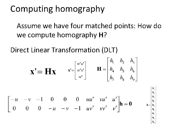
Computing homography Assume we have four matched points: How do we compute homography H? Direct Linear Transformation (DLT)

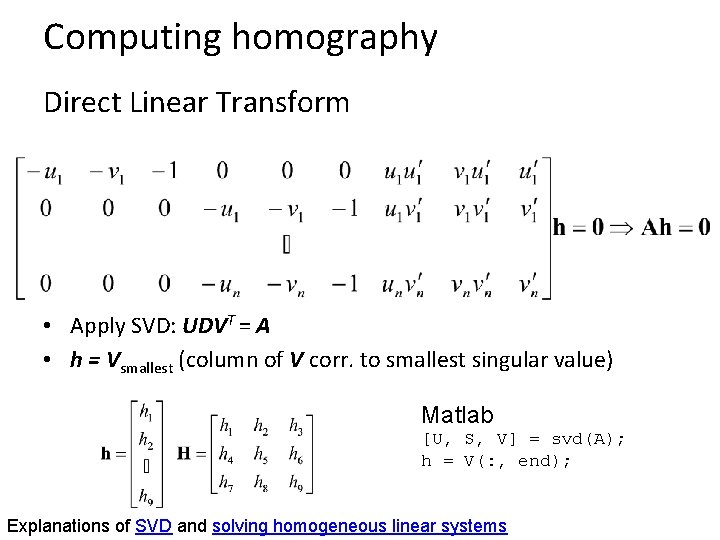
Computing homography Direct Linear Transform • Apply SVD: UDVT = A • h = Vsmallest (column of V corr. to smallest singular value) Matlab [U, S, V] = svd(A); h = V(: , end); Explanations of SVD and solving homogeneous linear systems

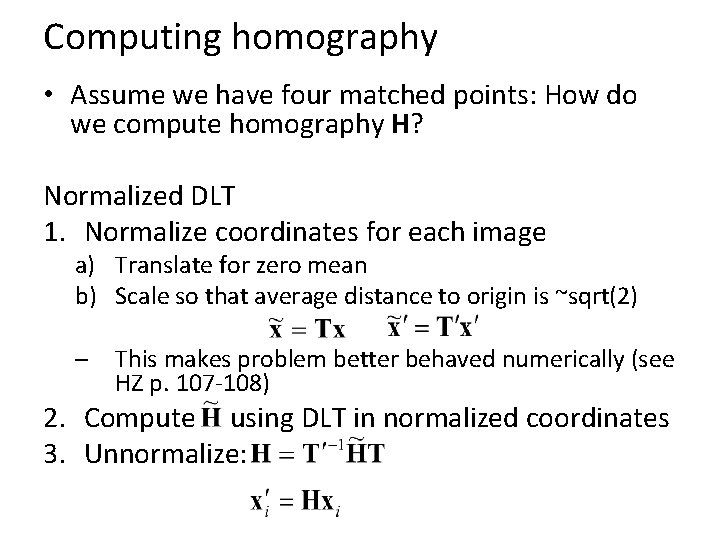
Computing homography • Assume we have four matched points: How do we compute homography H? Normalized DLT 1. Normalize coordinates for each image a) Translate for zero mean b) Scale so that average distance to origin is ~sqrt(2) – This makes problem better behaved numerically (see HZ p. 107 -108) 2. Compute using DLT in normalized coordinates 3. Unnormalize:

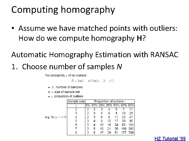
Computing homography • Assume we have matched points with outliers: How do we compute homography H? Automatic Homography Estimation with RANSAC 1. Choose number of samples N HZ Tutorial ‘ 99

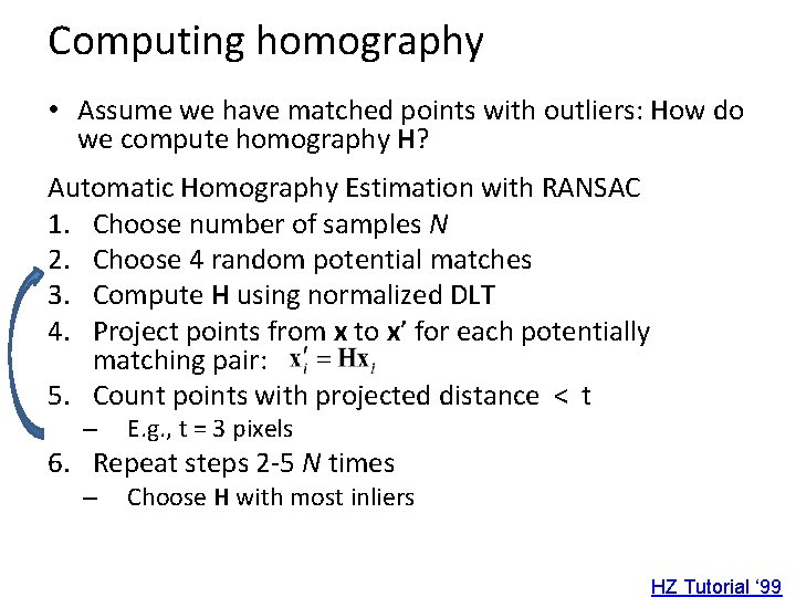
Computing homography • Assume we have matched points with outliers: How do we compute homography H? Automatic Homography Estimation with RANSAC 1. Choose number of samples N 2. Choose 4 random potential matches 3. Compute H using normalized DLT 4. Project points from x to x’ for each potentially matching pair: 5. Count points with projected distance < t – E. g. , t = 3 pixels 6. Repeat steps 2 -5 N times – Choose H with most inliers HZ Tutorial ‘ 99

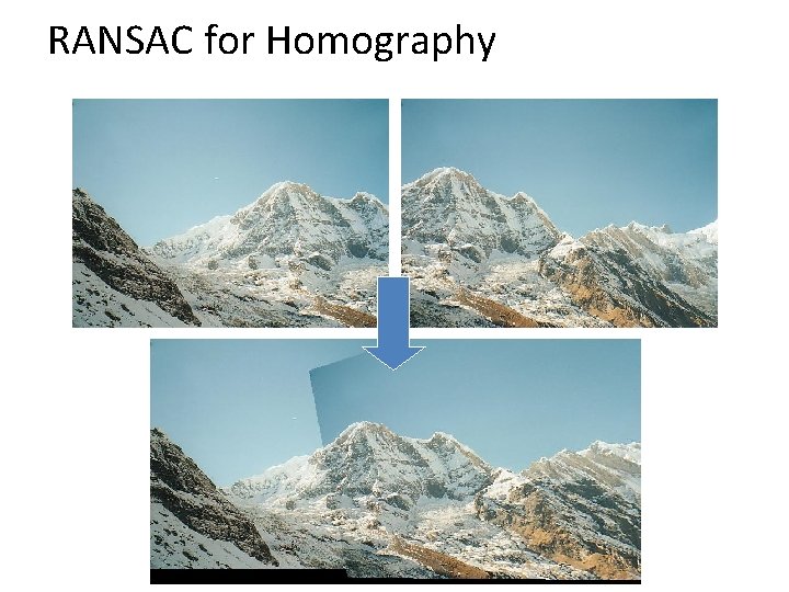
Automatic Image Stitching 1. Compute interest points on each image 2. Find candidate matches 3. Estimate homography H using matched points and RANSAC with normalized DLT 4. Project each image onto the same surface and blend – Matlab: maketform, imtransform

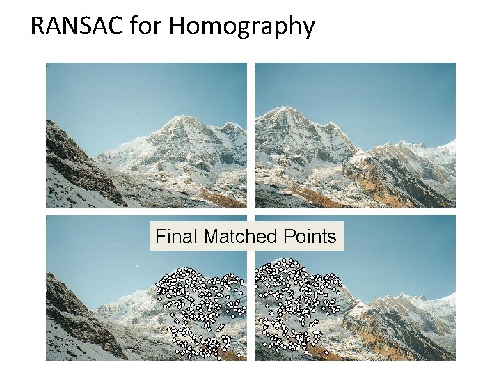
RANSAC for Homography Initial Matched Points

RANSAC for Homography Final Matched Points

RANSAC for Homography

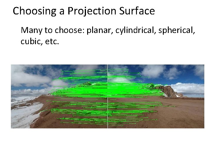
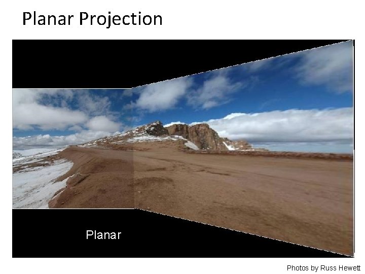
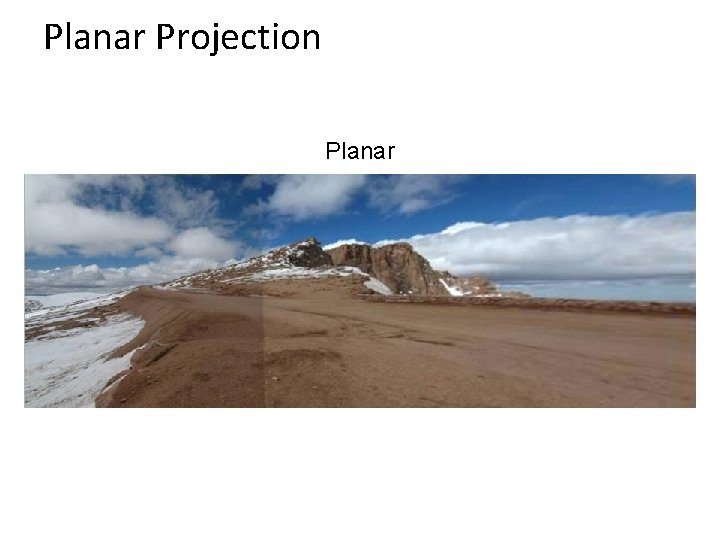
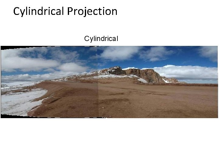
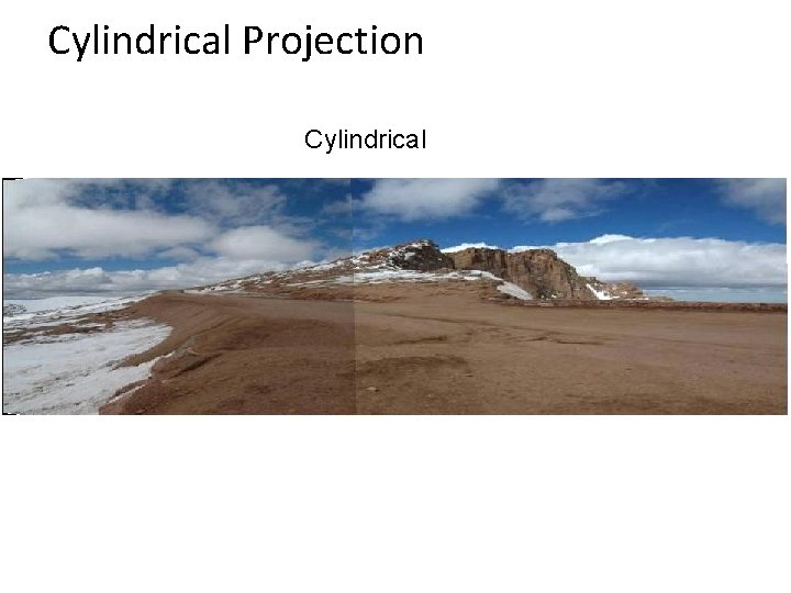
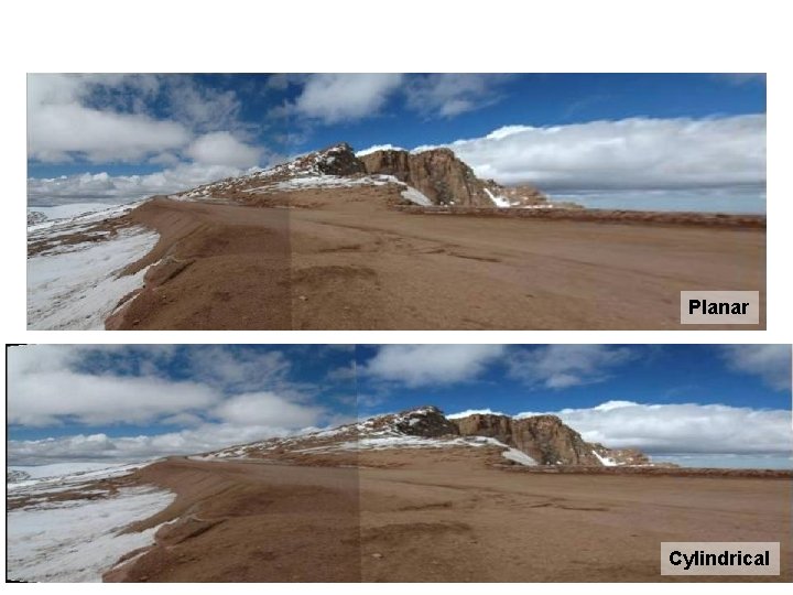
Choosing a Projection Surface Many to choose: planar, cylindrical, spherical, cubic, etc.

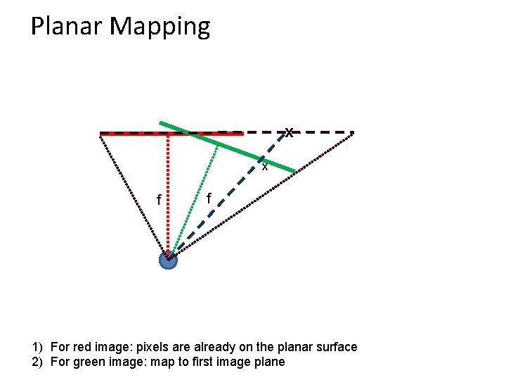
Planar Mapping x x f f 1) For red image: pixels are already on the planar surface 2) For green image: map to first image plane

Planar Projection Planar Photos by Russ Hewett

Planar Projection Planar

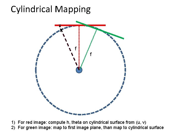
Cylindrical Mapping x x f f 1) For red image: compute h, theta on cylindrical surface from (u, v) 2) For green image: map to first image plane, than map to cylindrical surface

Cylindrical Projection Cylindrical

Cylindrical Projection Cylindrical

Planar Cylindrical

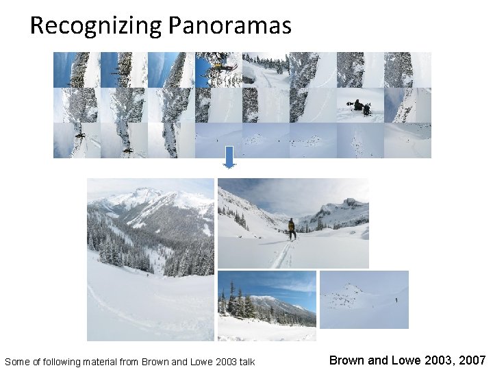
Recognizing Panoramas Some of following material from Brown and Lowe 2003 talk Brown and Lowe 2003, 2007

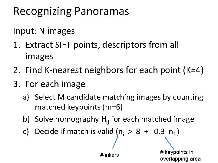
Recognizing Panoramas Input: N images 1. Extract SIFT points, descriptors from all images 2. Find K-nearest neighbors for each point (K=4) 3. For each image a) Select M candidate matching images by counting matched keypoints (m=6) b) Solve homography Hij for each matched image

Recognizing Panoramas Input: N images 1. Extract SIFT points, descriptors from all images 2. Find K-nearest neighbors for each point (K=4) 3. For each image a) Select M candidate matching images by counting matched keypoints (m=6) b) Solve homography Hij for each matched image c) Decide if match is valid (ni > 8 + 0. 3 nf ) # inliers # keypoints in overlapping area

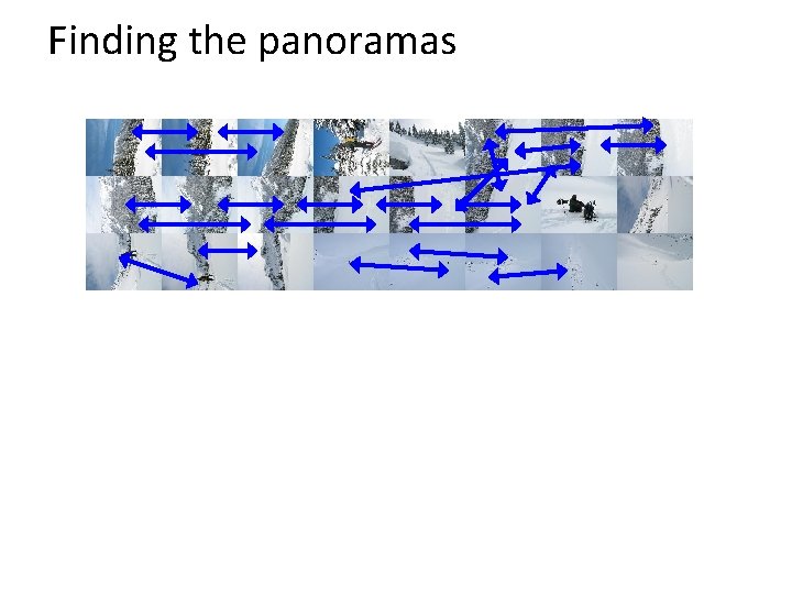
Recognizing Panoramas (cont. ) (now we have matched pairs of images) 4. Find connected components

Finding the panoramas

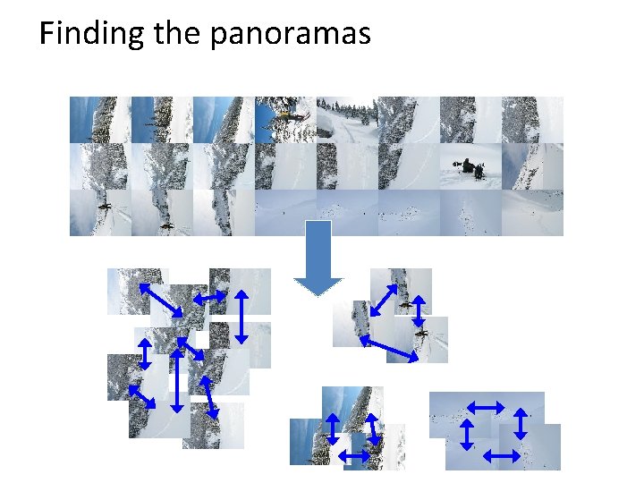
Finding the panoramas

Recognizing Panoramas (cont. ) (now we have matched pairs of images) 4. Find connected components 5. For each connected component a) Perform bundle adjustment to solve for rotation (θ 1, θ 2, θ 3) and focal length f of all cameras b) Project to a surface (plane, cylinder, or sphere) c) Render with multiband blending

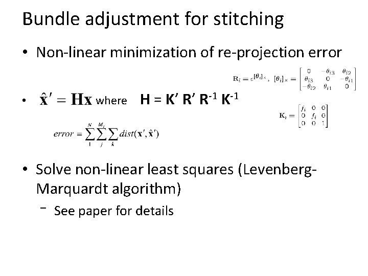
Bundle adjustment for stitching • Non-linear minimization of re-projection error where • H = K’ R’ R-1 K-1 • Solve non-linear least squares (Levenberg. Marquardt algorithm) – See paper for details

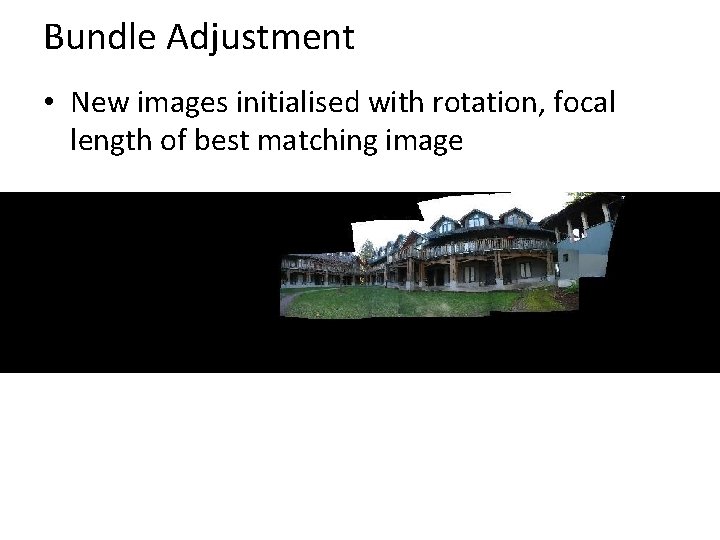
Bundle Adjustment • New images initialised with rotation, focal length of best matching image

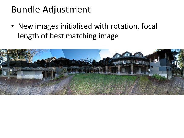
Bundle Adjustment • New images initialised with rotation, focal length of best matching image

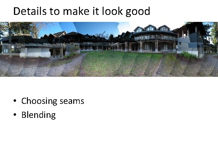
Details to make it look good • Choosing seams • Blending

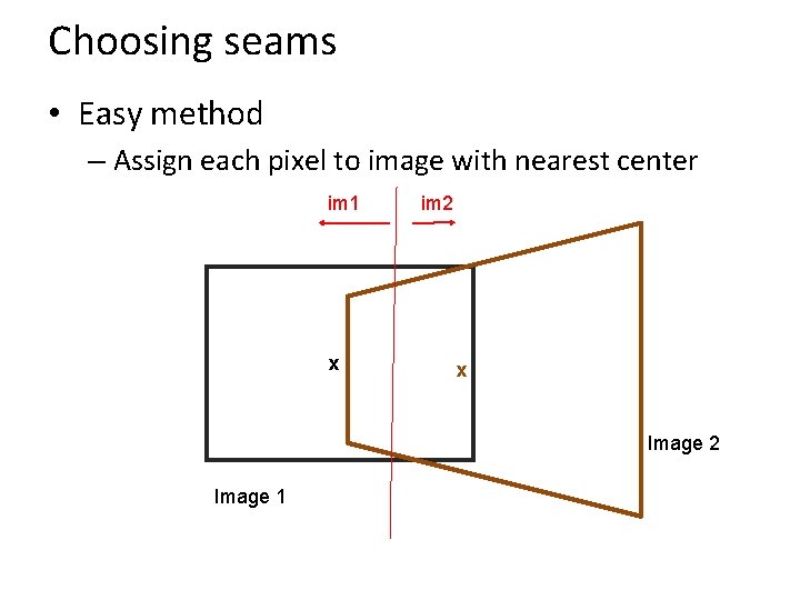
Choosing seams • Easy method – Assign each pixel to image with nearest center im 1 x im 2 x Image 2 Image 1

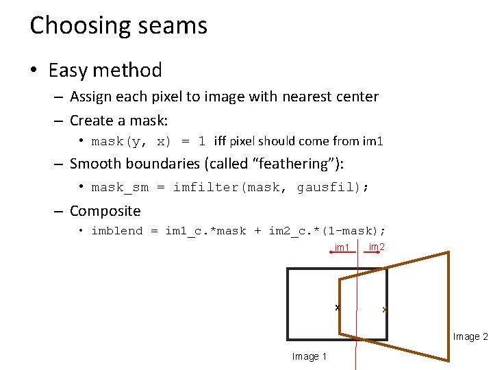
Choosing seams • Easy method – Assign each pixel to image with nearest center – Create a mask: • mask(y, x) = 1 iff pixel should come from im 1 – Smooth boundaries (called “feathering”): • mask_sm = imfilter(mask, gausfil); – Composite • imblend = im 1_c. *mask + im 2_c. *(1 -mask); im 1 x im 2 x Image 2 Image 1

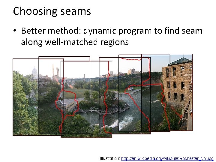
Choosing seams • Better method: dynamic program to find seam along well-matched regions Illustration: http: //en. wikipedia. org/wiki/File: Rochester_NY. jpg

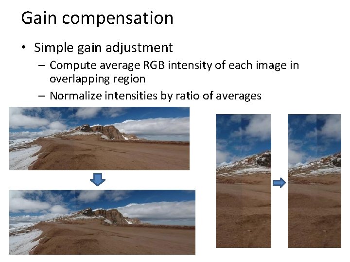
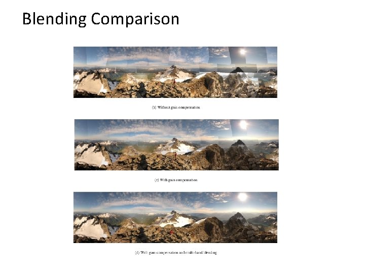
Gain compensation • Simple gain adjustment – Compute average RGB intensity of each image in overlapping region – Normalize intensities by ratio of averages

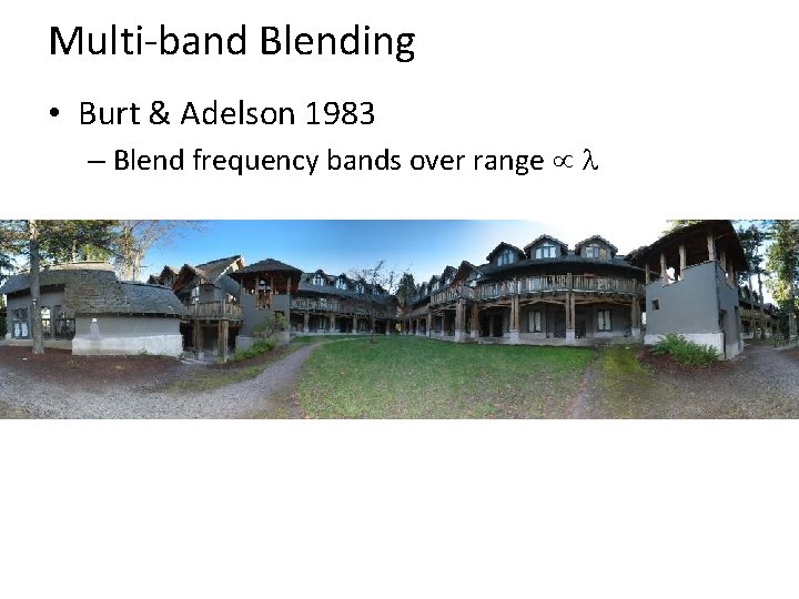
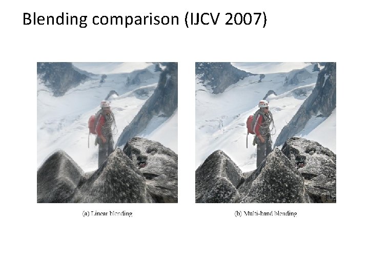
Multi-band Blending • Burt & Adelson 1983 – Blend frequency bands over range l

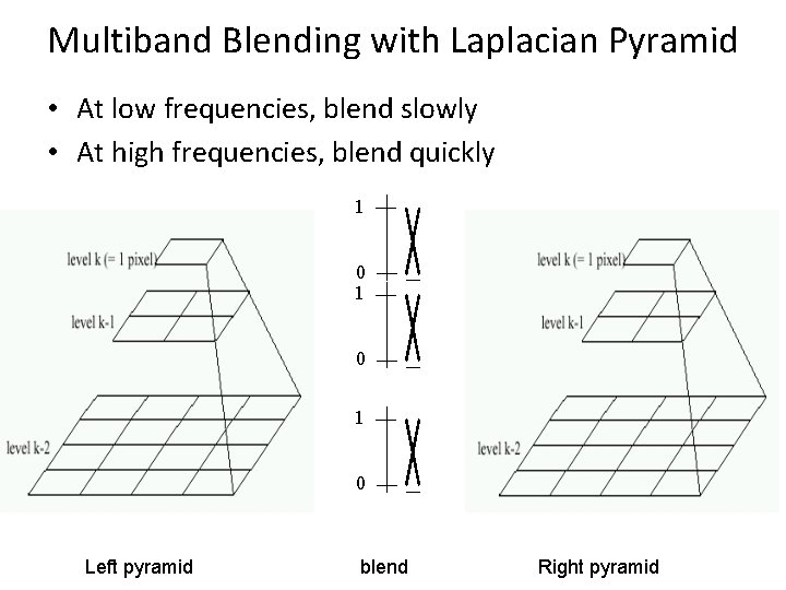
Multiband Blending with Laplacian Pyramid • At low frequencies, blend slowly • At high frequencies, blend quickly 1 0 1 0 Left pyramid blend Right pyramid

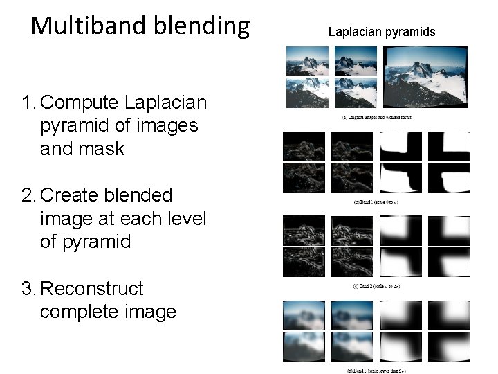
Multiband blending 1. Compute Laplacian pyramid of images and mask 2. Create blended image at each level of pyramid 3. Reconstruct complete image Laplacian pyramids

Blending comparison (IJCV 2007)

Blending Comparison

Further reading • DLT algorithm: HZ p. 91 (alg 4. 2), p. 585 • Normalization: HZ p. 107 -109 (alg 4. 2) • RANSAC: HZ Sec 4. 7, p. 123, alg 4. 6 • Rick Szeliski’s alignment/stitching tutorial • Recognising Panoramas: Brown and Lowe, IJCV 2007 (also bundle adjustment)

Things to remember • Homography relates rotating cameras • Recover homography using RANSAC and normalized DLT • Bundle adjustment minimizes reprojection error for set of related images • Details to make it look nice (e. g. , blending)

Next class • Stereo and epipolar geometry