012412 Pixels and Image Filtering Computer Vision Derek

01/24/12 Pixels and Image Filtering Computer Vision Derek Hoiem, University of Illinois Graphic: http: //www. notcot. org/post/4068/

Today’s Class: Pixels and Linear Filters • Review of lighting – Reflection and absorption • What is image filtering and how do we do it? • Color models (if time allows)

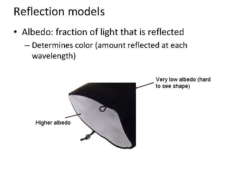
Reflection models • Albedo: fraction of light that is reflected – Determines color (amount reflected at each wavelength) Very low albedo (hard to see shape) Higher albedo

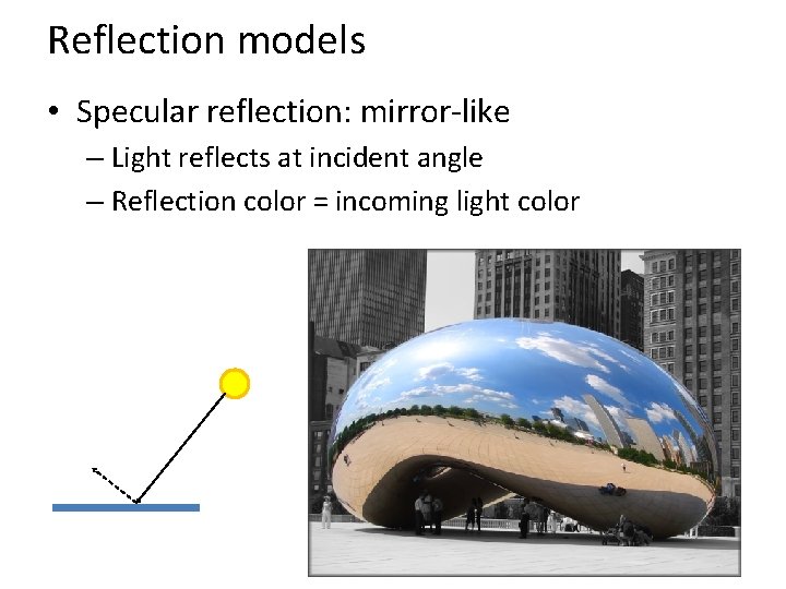
Reflection models • Specular reflection: mirror-like – Light reflects at incident angle – Reflection color = incoming light color

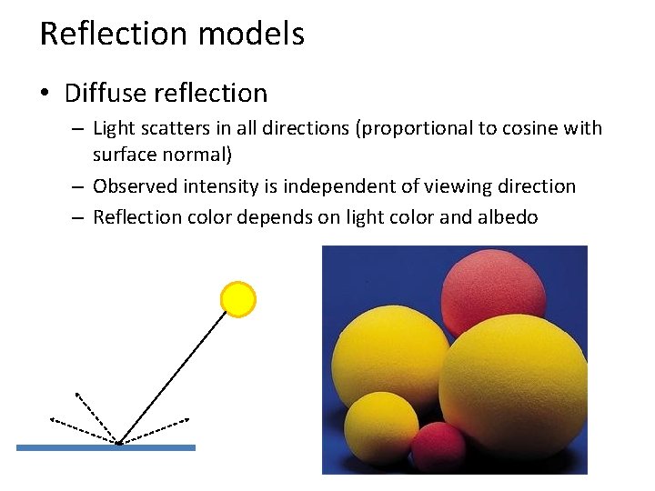
Reflection models • Diffuse reflection – Light scatters in all directions (proportional to cosine with surface normal) – Observed intensity is independent of viewing direction – Reflection color depends on light color and albedo

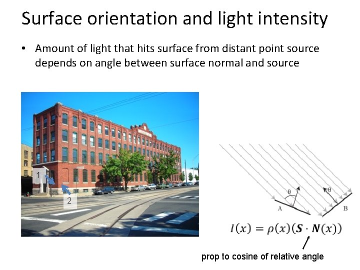
Surface orientation and light intensity • Amount of light that hits surface from distant point source depends on angle between surface normal and source 1 2 prop to cosine of relative angle

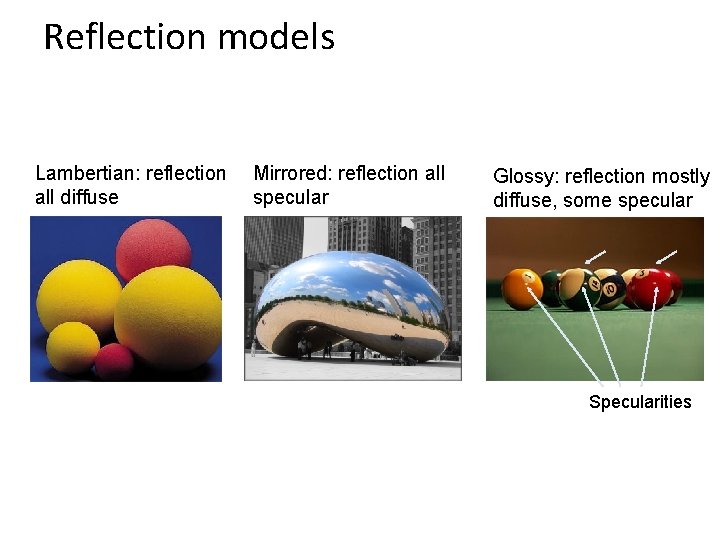
Reflection models Lambertian: reflection all diffuse Mirrored: reflection all specular Glossy: reflection mostly diffuse, some specular Specularities

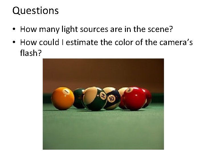
Questions • How many light sources are in the scene? • How could I estimate the color of the camera’s flash?

The plight of the poor pixel • A pixel’s brightness is determined by – Light source (strength, direction, color) – Surface orientation – Surface material and albedo – Reflected light and shadows from surrounding surfaces – Gain on the sensor • A pixel’s brightness tells us nothing by itself

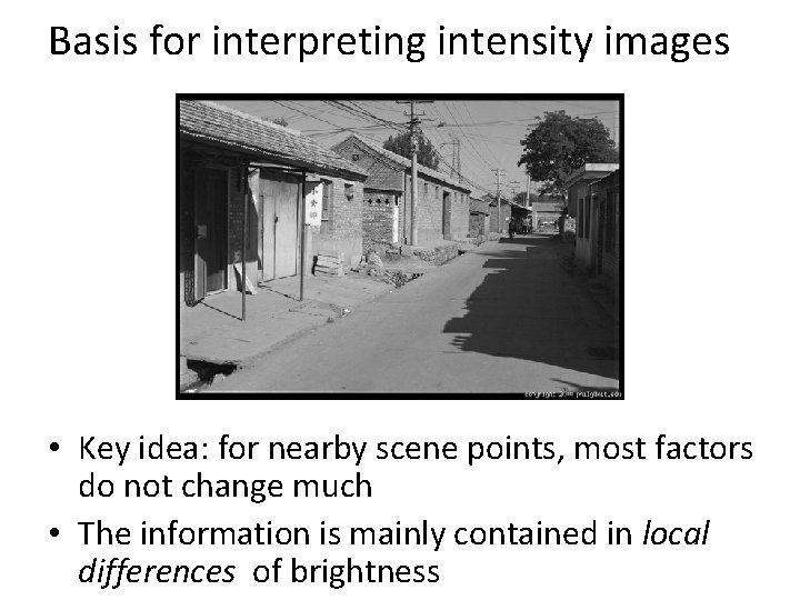
Basis for interpreting intensity images • Key idea: for nearby scene points, most factors do not change much • The information is mainly contained in local differences of brightness

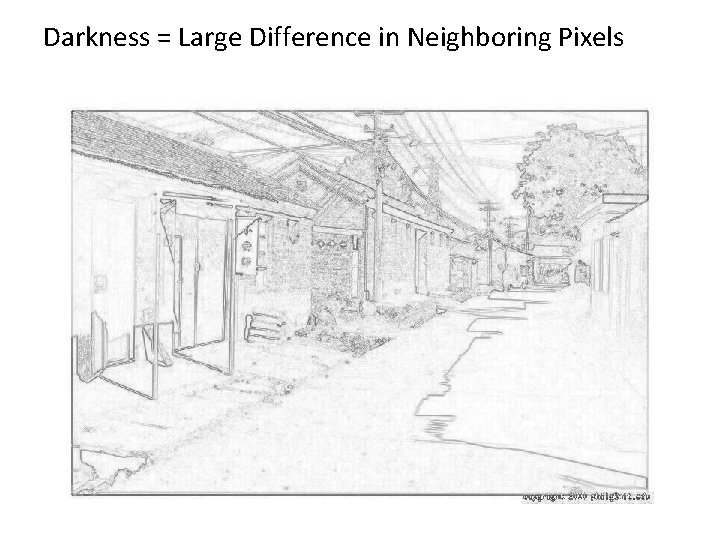
Darkness = Large Difference in Neighboring Pixels

Next three classes: three views of filtering • Image filters in spatial domain – Filter is a mathematical operation of a grid of numbers – Smoothing, sharpening, measuring texture • Image filters in the frequency domain – Filtering is a way to modify the frequencies of images – Denoising, sampling, image compression • Templates and Image Pyramids – Filtering is a way to match a template to the image – Detection, coarse-to-fine registration

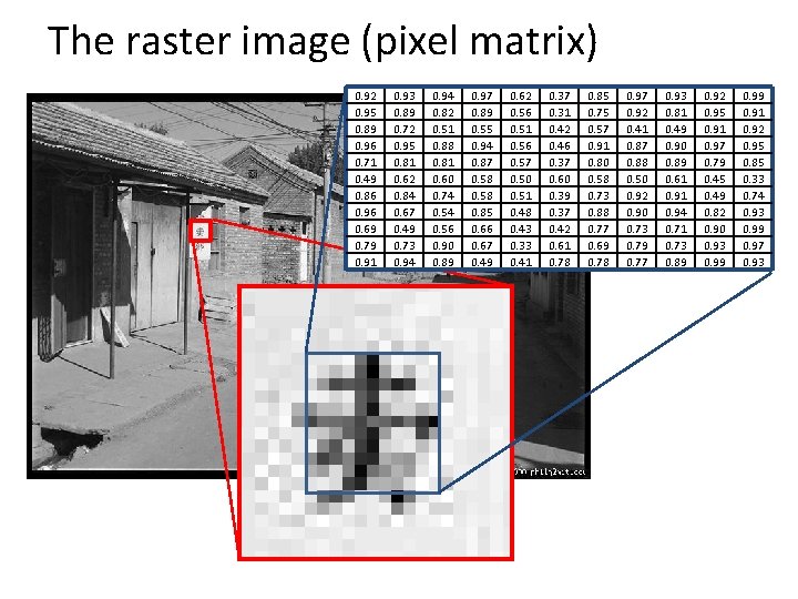
The raster image (pixel matrix) 0. 92 0. 95 0. 89 0. 96 0. 71 0. 49 0. 86 0. 96 0. 69 0. 79 0. 91 0. 93 0. 89 0. 72 0. 95 0. 81 0. 62 0. 84 0. 67 0. 49 0. 73 0. 94 0. 82 0. 51 0. 88 0. 81 0. 60 0. 74 0. 56 0. 90 0. 89 0. 97 0. 89 0. 55 0. 94 0. 87 0. 58 0. 85 0. 66 0. 67 0. 49 0. 62 0. 56 0. 51 0. 56 0. 57 0. 50 0. 51 0. 48 0. 43 0. 33 0. 41 0. 37 0. 31 0. 42 0. 46 0. 37 0. 60 0. 39 0. 37 0. 42 0. 61 0. 78 0. 85 0. 75 0. 57 0. 91 0. 80 0. 58 0. 73 0. 88 0. 77 0. 69 0. 78 0. 97 0. 92 0. 41 0. 87 0. 88 0. 50 0. 92 0. 90 0. 73 0. 79 0. 77 0. 93 0. 81 0. 49 0. 90 0. 89 0. 61 0. 94 0. 71 0. 73 0. 89 0. 92 0. 95 0. 91 0. 97 0. 79 0. 45 0. 49 0. 82 0. 90 0. 93 0. 99 0. 91 0. 92 0. 95 0. 85 0. 33 0. 74 0. 93 0. 99 0. 97 0. 93

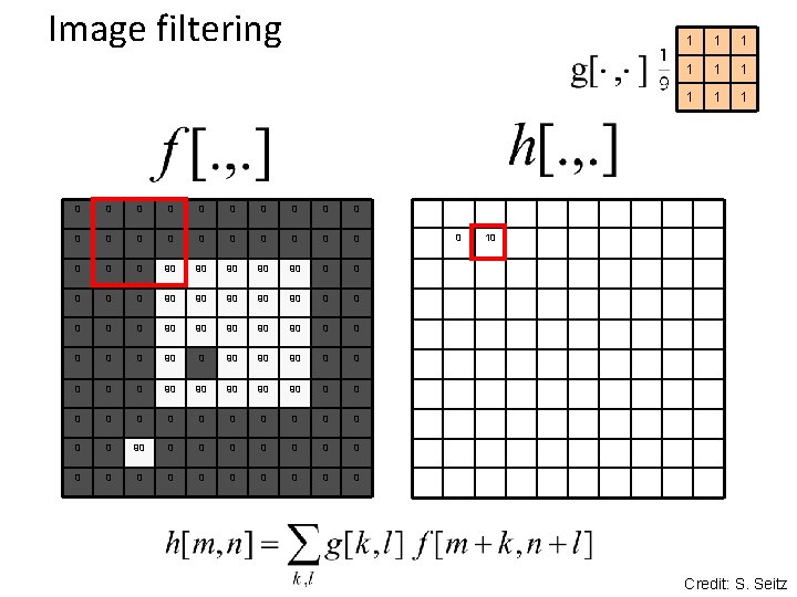
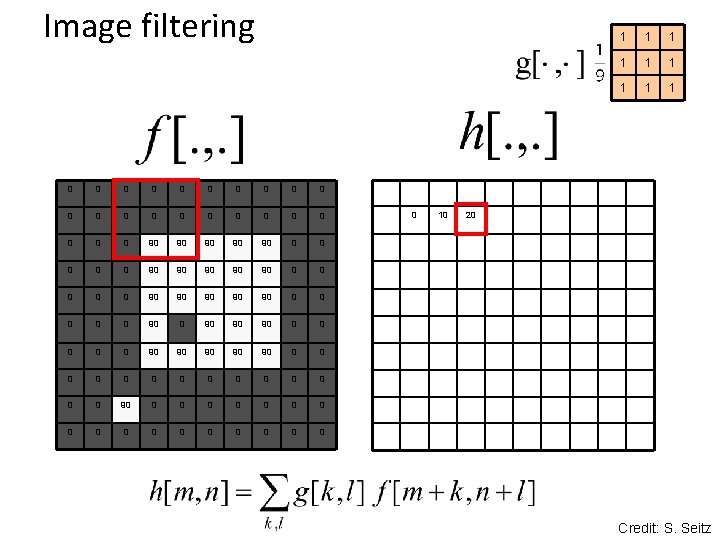
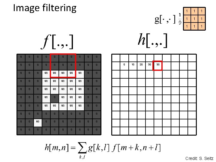
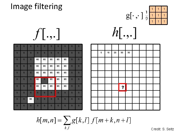
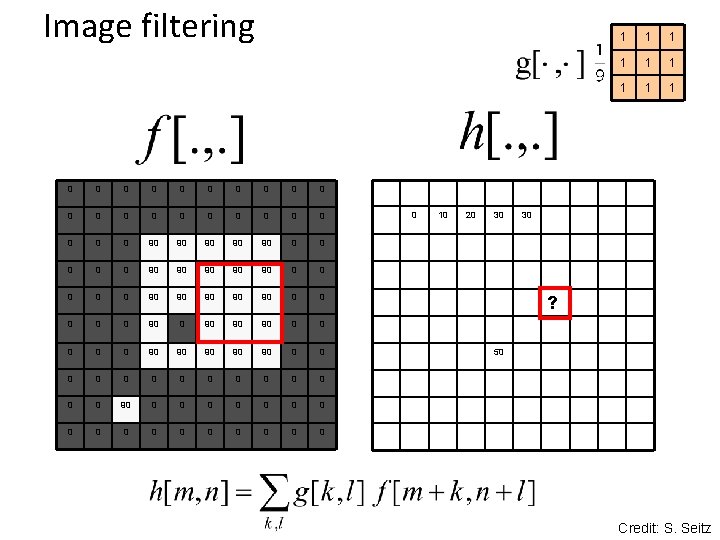
Image filtering • Image filtering: compute function of local neighborhood at each position • Linear filtering: function is a weighted sum/difference of pixel values • Really important! – Enhance images • Denoise, resize, increase contrast, etc. – Extract information from images • Texture, edges, distinctive points, etc. – Detect patterns • Template matching

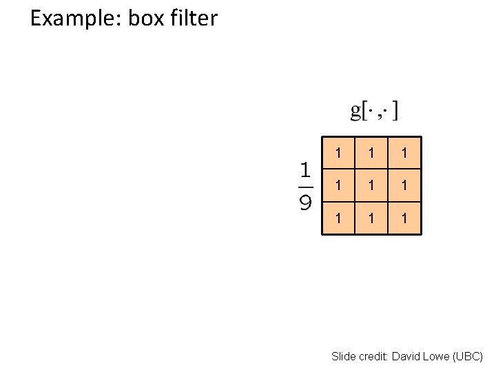
Example: box filter 1 1 1 1 1 Slide credit: David Lowe (UBC)

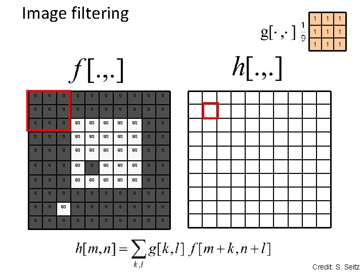
Image filtering 0 0 0 0 0 0 90 90 90 0 0 90 90 90 0 0 0 0 90 90 90 0 0 90 90 90 0 0 0 0 0 0 0 90 90 0 0 0 0 0 0 0 0 1 1 1 1 1 0 Credit: S. Seitz

Image filtering 0 0 0 0 0 0 90 90 90 0 0 90 90 90 0 90 90 90 0 0 0 0 0 0 0 0 0 1 1 10 Credit: S. Seitz

Image filtering 0 0 0 0 0 0 90 90 90 0 0 90 90 90 0 90 90 90 0 0 0 0 0 0 0 0 0 10 1 1 1 1 1 20 Credit: S. Seitz

Image filtering 0 0 0 0 0 0 90 90 90 0 0 90 90 90 0 90 90 90 0 0 0 0 0 0 0 0 0 10 20 1 1 1 1 1 30 Credit: S. Seitz

Image filtering 0 0 0 0 0 0 90 90 90 0 0 90 90 90 0 90 90 90 0 0 0 0 0 0 0 0 0 10 20 30 1 1 1 1 1 30 Credit: S. Seitz

Image filtering 0 0 0 0 0 0 90 90 90 0 0 90 90 90 0 90 90 90 0 0 0 0 0 0 0 0 0 10 20 30 1 1 1 1 1 30 ? Credit: S. Seitz

Image filtering 0 0 0 0 0 0 90 90 90 0 0 90 90 90 0 90 90 90 0 0 0 0 0 0 0 0 0 10 20 30 1 1 1 1 1 30 ? 50 Credit: S. Seitz

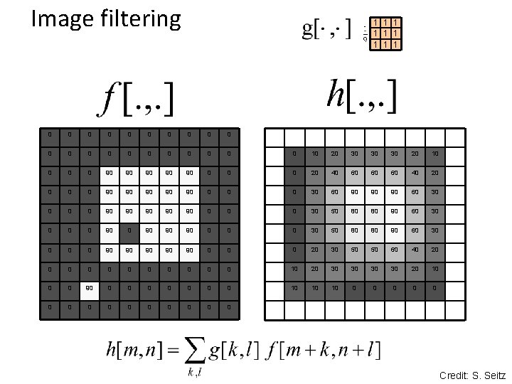
Image filtering 1 1 1 1 1 0 0 0 0 0 0 10 20 30 30 30 20 10 0 90 90 90 0 20 40 60 60 60 40 20 0 90 90 90 0 30 60 90 90 90 60 30 0 90 90 90 0 30 50 80 80 90 60 30 0 90 90 90 0 20 30 50 50 60 40 20 0 0 10 20 30 30 20 10 0 0 90 0 0 0 10 10 10 0 0 0 Credit: S. Seitz

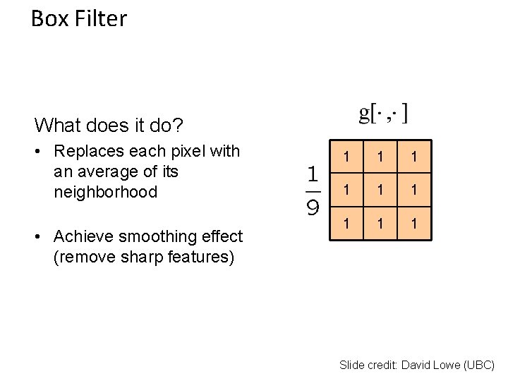
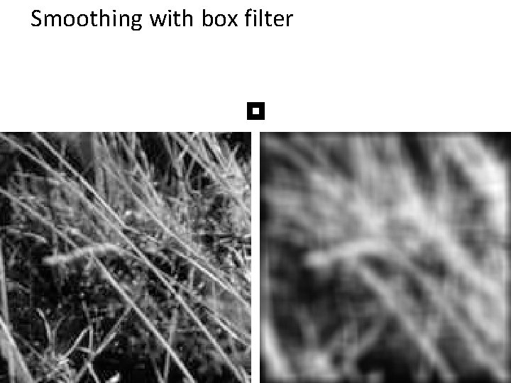
Box Filter What does it do? • Replaces each pixel with an average of its neighborhood • Achieve smoothing effect (remove sharp features) 1 1 1 1 1 Slide credit: David Lowe (UBC)

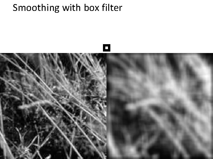
Smoothing with box filter

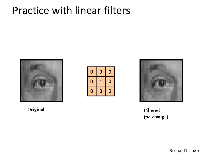
Practice with linear filters 0 0 1 0 0 ? Original Source: D. Lowe

Practice with linear filters Original 0 0 1 0 0 Filtered (no change) Source: D. Lowe

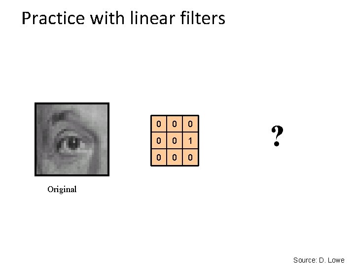
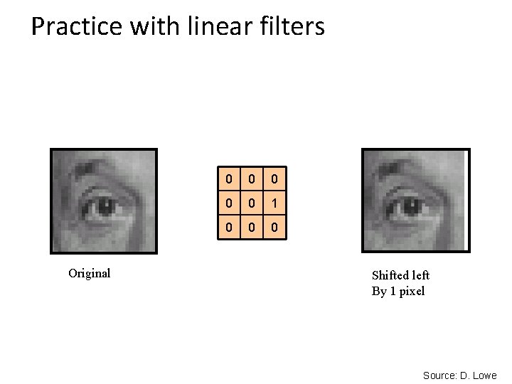
Practice with linear filters 0 0 0 1 0 0 0 ? Original Source: D. Lowe

Practice with linear filters Original 0 0 0 1 0 0 0 Shifted left By 1 pixel Source: D. Lowe

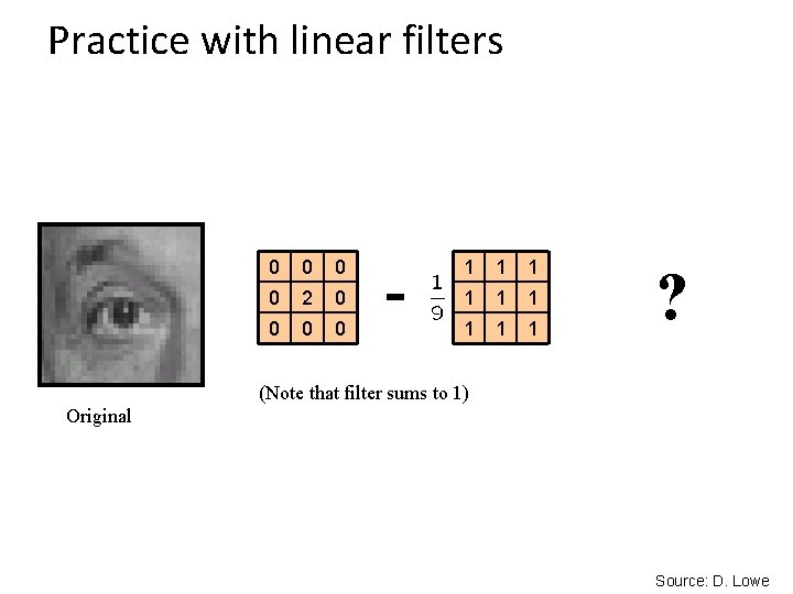
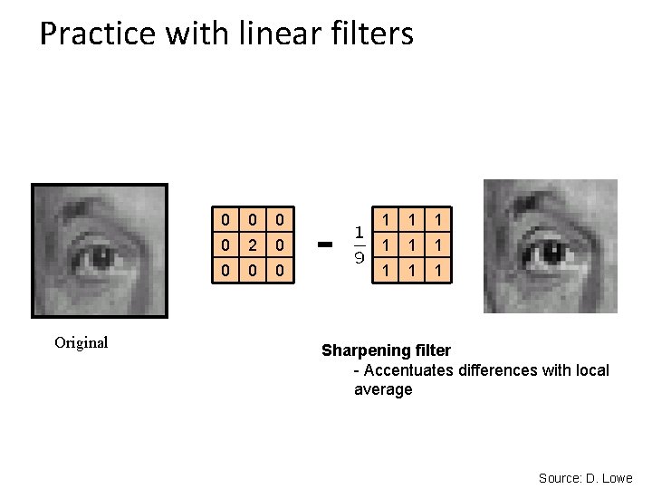
Practice with linear filters 0 0 2 0 0 - 1 1 1 1 1 ? (Note that filter sums to 1) Original Source: D. Lowe

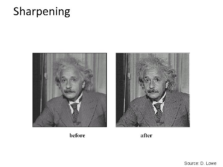
Practice with linear filters Original 0 0 2 0 0 - 1 1 1 1 1 Sharpening filter - Accentuates differences with local average Source: D. Lowe

Sharpening Source: D. Lowe

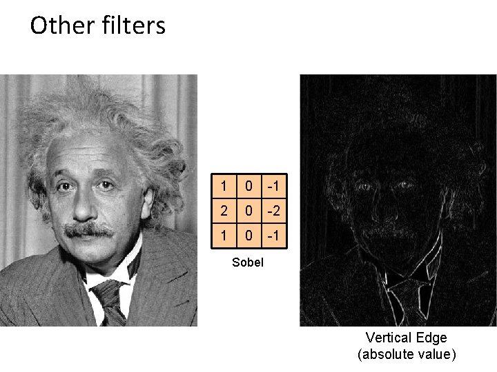
Other filters 1 0 -1 2 0 -2 1 0 -1 Sobel Vertical Edge (absolute value)

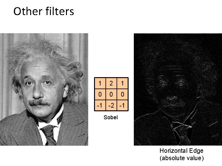
Other filters 1 2 1 0 0 0 -1 -2 -1 Sobel Horizontal Edge (absolute value)

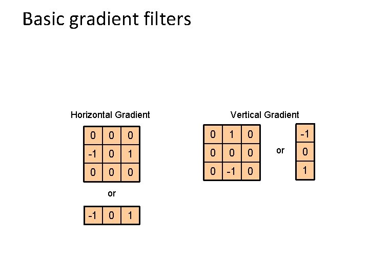
Basic gradient filters Horizontal Gradient Vertical Gradient 0 0 1 0 -1 0 0 0 0 -1 0 or -1 0 1 -1 or 0 1

Example

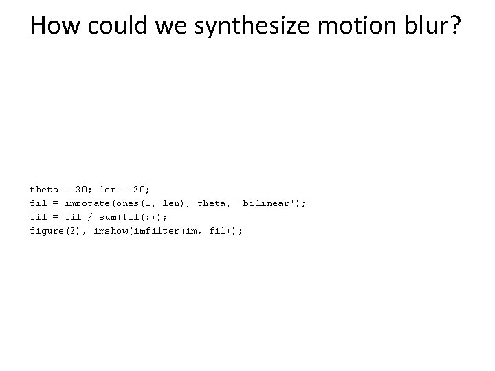
How could we synthesize motion blur? theta = 30; len = 20; fil = imrotate(ones(1, len), theta, 'bilinear'); fil = fil / sum(fil(: )); figure(2), imshow(imfilter(im, fil));

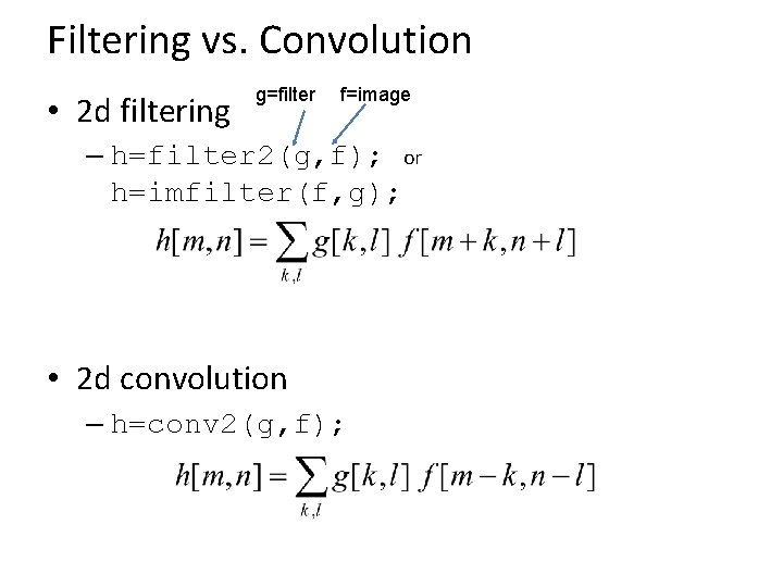
Filtering vs. Convolution • 2 d filtering g=filter f=image – h=filter 2(g, f); or h=imfilter(f, g); • 2 d convolution – h=conv 2(g, f);

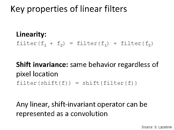
Key properties of linear filters Linearity: filter(f 1 + f 2) = filter(f 1) + filter(f 2) Shift invariance: same behavior regardless of pixel location filter(shift(f)) = shift(filter(f)) Any linear, shift-invariant operator can be represented as a convolution Source: S. Lazebnik

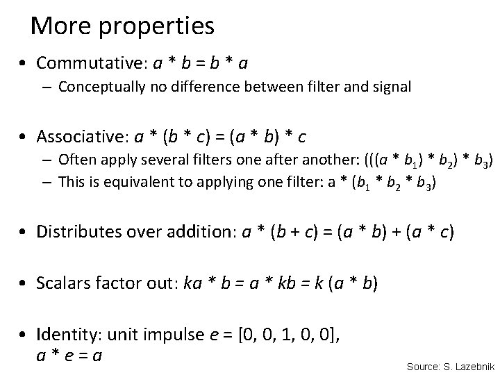
More properties • Commutative: a * b = b * a – Conceptually no difference between filter and signal • Associative: a * (b * c) = (a * b) * c – Often apply several filters one after another: (((a * b 1) * b 2) * b 3) – This is equivalent to applying one filter: a * (b 1 * b 2 * b 3) • Distributes over addition: a * (b + c) = (a * b) + (a * c) • Scalars factor out: ka * b = a * kb = k (a * b) • Identity: unit impulse e = [0, 0, 1, 0, 0], a*e=a Source: S. Lazebnik

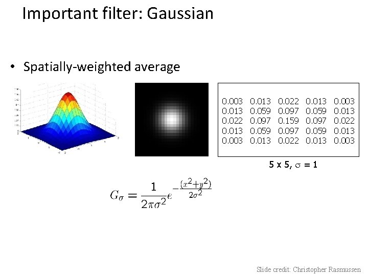
Important filter: Gaussian • Spatially-weighted average 0. 003 0. 013 0. 022 0. 013 0. 003 0. 013 0. 059 0. 097 0. 059 0. 013 0. 022 0. 097 0. 159 0. 097 0. 022 0. 013 0. 059 0. 097 0. 059 0. 013 0. 003 0. 013 0. 022 0. 013 0. 003 5 x 5, = 1 Slide credit: Christopher Rasmussen

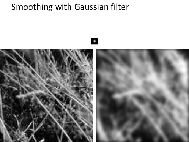
Smoothing with Gaussian filter

Smoothing with box filter

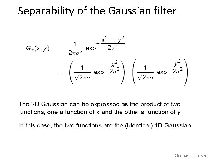
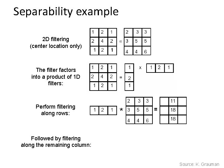
Gaussian filters • Remove “high-frequency” components from the image (low-pass filter) – Images become more smooth • Convolution with self is another Gaussian – So can smooth with small-width kernel, repeat, and get same result as larger-width kernel would have – Convolving two times with Gaussian kernel of width σ is same as convolving once with kernel of width σ√ 2 • Separable kernel – Factors into product of two 1 D Gaussians Source: K. Grauman

Separability of the Gaussian filter Source: D. Lowe

Separability example 2 D filtering (center location only) The filter factors into a product of 1 D filters: Perform filtering along rows: Followed by filtering along the remaining column: * = Source: K. Grauman

Separability • Why is separability useful in practice?

Some practical matters

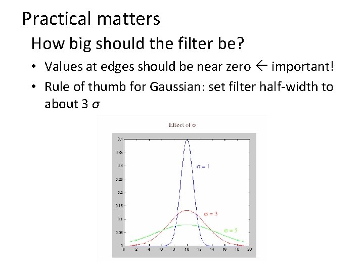
Practical matters How big should the filter be? • Values at edges should be near zero important! • Rule of thumb for Gaussian: set filter half-width to about 3 σ

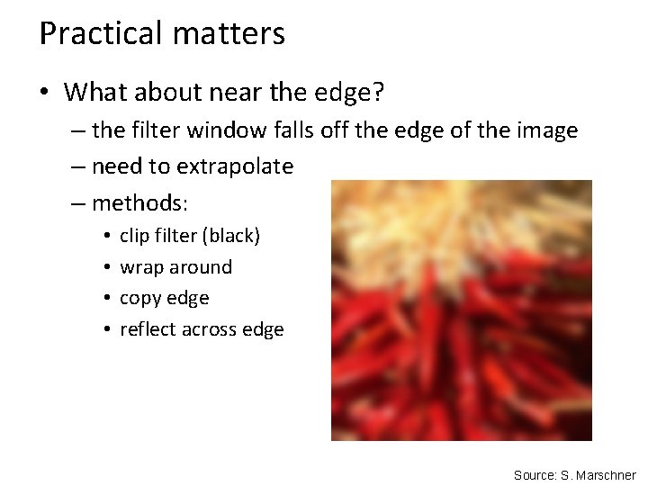
Practical matters • What about near the edge? – the filter window falls off the edge of the image – need to extrapolate – methods: • • clip filter (black) wrap around copy edge reflect across edge Source: S. Marschner

Practical matters – methods (MATLAB): • • clip filter (black): wrap around: copy edge: reflect across edge: imfilter(f, g, 0) imfilter(f, g, ‘circular’) imfilter(f, g, ‘replicate’) imfilter(f, g, ‘symmetric’) Source: S. Marschner

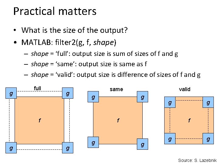
Practical matters • What is the size of the output? • MATLAB: filter 2(g, f, shape) – shape = ‘full’: output size is sum of sizes of f and g – shape = ‘same’: output size is same as f – shape = ‘valid’: output size is difference of sizes of f and g g full g same g f g valid g g f g g g Source: S. Lazebnik

A little more about color…

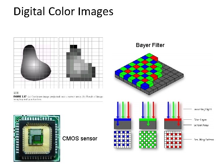
Digital Color Images Bayer Filter CMOS sensor

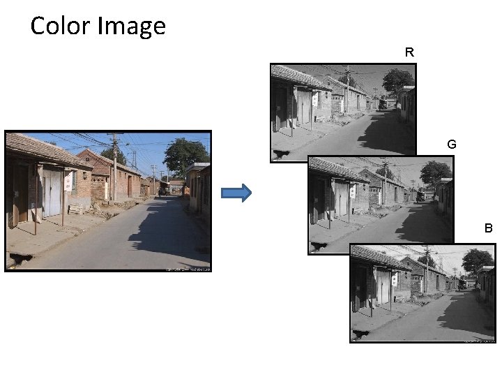
Color Image R G B

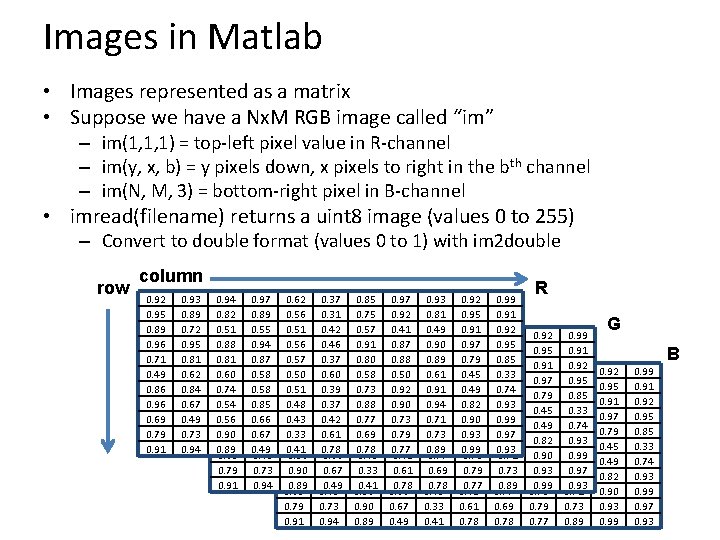
Images in Matlab • Images represented as a matrix • Suppose we have a Nx. M RGB image called “im” – im(1, 1, 1) = top-left pixel value in R-channel – im(y, x, b) = y pixels down, x pixels to right in the bth channel – im(N, M, 3) = bottom-right pixel in B-channel • imread(filename) returns a uint 8 image (values 0 to 255) – Convert to double format (values 0 to 1) with im 2 double row column 0. 92 0. 95 0. 89 0. 96 0. 71 0. 49 0. 86 0. 96 0. 69 0. 79 0. 91 0. 93 0. 89 0. 72 0. 95 0. 81 0. 62 0. 84 0. 67 0. 49 0. 73 0. 94 0. 82 0. 51 0. 92 0. 88 0. 95 0. 81 0. 89 0. 60 0. 96 0. 74 0. 71 0. 54 0. 49 0. 56 0. 86 0. 90 0. 96 0. 89 0. 69 0. 79 0. 91 0. 97 0. 89 0. 55 0. 93 0. 94 0. 89 0. 87 0. 72 0. 58 0. 95 0. 58 0. 81 0. 85 0. 62 0. 66 0. 84 0. 67 0. 49 0. 73 0. 94 0. 62 0. 56 0. 51 0. 94 0. 56 0. 82 0. 57 0. 51 0. 92 0. 50 0. 88 0. 95 0. 51 0. 89 0. 48 0. 60 0. 96 0. 43 0. 74 0. 71 0. 33 0. 54 0. 49 0. 41 0. 56 0. 86 0. 90 0. 96 0. 89 0. 69 0. 79 0. 91 0. 37 0. 31 0. 42 0. 97 0. 46 0. 89 0. 37 0. 55 0. 93 0. 60 0. 94 0. 89 0. 39 0. 87 0. 72 0. 37 0. 58 0. 95 0. 42 0. 58 0. 81 0. 61 0. 85 0. 62 0. 78 0. 66 0. 84 0. 67 0. 49 0. 73 0. 94 0. 85 0. 75 0. 57 0. 62 0. 91 0. 56 0. 80 0. 51 0. 94 0. 58 0. 56 0. 82 0. 73 0. 57 0. 51 0. 88 0. 50 0. 88 0. 77 0. 51 0. 81 0. 69 0. 48 0. 60 0. 78 0. 43 0. 74 0. 33 0. 54 0. 41 0. 56 0. 90 0. 89 0. 97 0. 92 0. 41 0. 37 0. 87 0. 31 0. 88 0. 42 0. 97 0. 50 0. 46 0. 89 0. 92 0. 37 0. 55 0. 90 0. 60 0. 94 0. 73 0. 39 0. 87 0. 79 0. 37 0. 58 0. 77 0. 42 0. 58 0. 61 0. 85 0. 78 0. 66 0. 67 0. 49 0. 93 0. 81 0. 49 0. 85 0. 90 0. 75 0. 89 0. 57 0. 62 0. 61 0. 91 0. 56 0. 91 0. 80 0. 51 0. 94 0. 58 0. 56 0. 71 0. 73 0. 57 0. 73 0. 88 0. 50 0. 89 0. 77 0. 51 0. 69 0. 48 0. 78 0. 43 0. 33 0. 41 0. 92 0. 95 0. 91 0. 97 0. 92 0. 79 0. 41 0. 37 0. 45 0. 87 0. 31 0. 49 0. 88 0. 42 0. 82 0. 50 0. 46 0. 90 0. 92 0. 37 0. 93 0. 90 0. 60 0. 99 0. 73 0. 39 0. 79 0. 37 0. 77 0. 42 0. 61 0. 78 0. 99 0. 91 0. 92 0. 93 0. 95 0. 81 0. 85 0. 49 0. 85 0. 33 0. 90 0. 75 0. 74 0. 89 0. 57 0. 93 0. 61 0. 99 0. 91 0. 80 0. 97 0. 94 0. 58 0. 93 0. 71 0. 73 0. 88 0. 89 0. 77 0. 69 0. 78 R 0. 92 0. 95 0. 91 0. 97 0. 92 0. 79 0. 41 0. 45 0. 87 0. 49 0. 88 0. 82 0. 50 0. 92 0. 93 0. 90 0. 99 0. 73 0. 79 0. 77 0. 99 0. 91 0. 92 0. 93 0. 95 0. 81 0. 85 0. 49 0. 33 0. 90 0. 74 0. 89 0. 93 0. 61 0. 99 0. 91 0. 97 0. 94 0. 93 0. 71 0. 73 0. 89 G B 0. 92 0. 95 0. 91 0. 97 0. 79 0. 45 0. 49 0. 82 0. 90 0. 93 0. 99 0. 91 0. 92 0. 95 0. 85 0. 33 0. 74 0. 93 0. 99 0. 97 0. 93

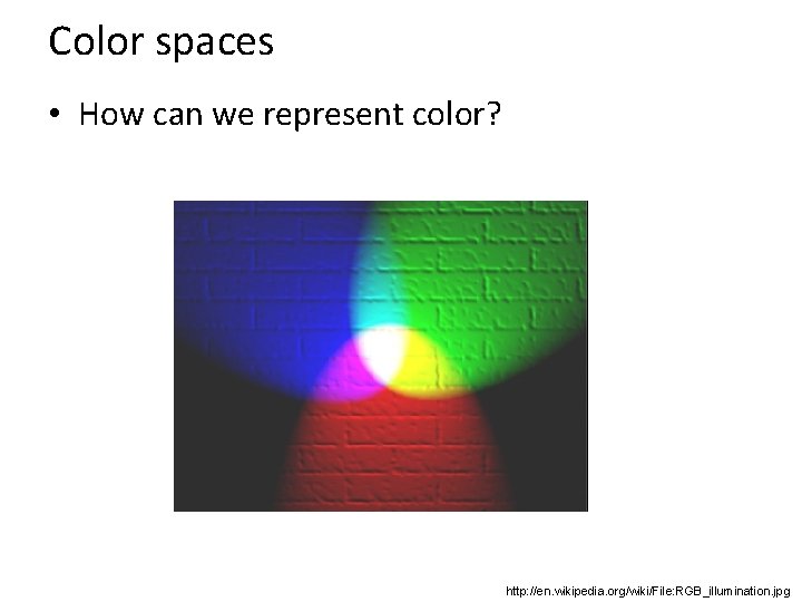
Color spaces • How can we represent color? http: //en. wikipedia. org/wiki/File: RGB_illumination. jpg

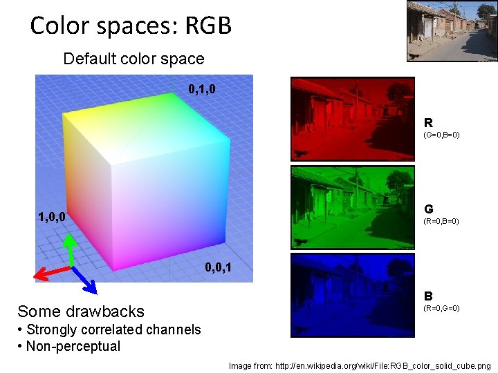
Color spaces: RGB Default color space 0, 1, 0 R (G=0, B=0) G 1, 0, 0 (R=0, B=0) 0, 0, 1 Some drawbacks B (R=0, G=0) • Strongly correlated channels • Non-perceptual Image from: http: //en. wikipedia. org/wiki/File: RGB_color_solid_cube. png

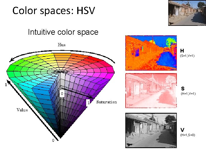
Color spaces: HSV Intuitive color space H (S=1, V=1) S (H=1, V=1) V (H=1, S=0)

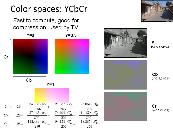
Color spaces: YCb. Cr Fast to compute, good for compression, used by TV Y=0. 5 Y (Cb=0. 5, Cr=0. 5) Cr Cb Cb (Y=0. 5, Cr=0. 5) Y=1 Cr (Y=0. 5, Cb=05)

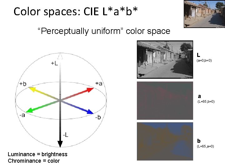
Color spaces: CIE L*a*b* “Perceptually uniform” color space L (a=0, b=0) a (L=65, b=0) b (L=65, a=0) Luminance = brightness Chrominance = color

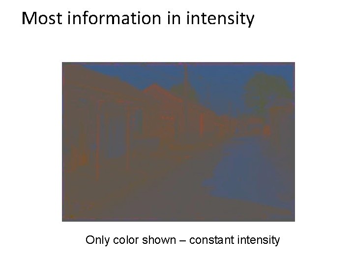
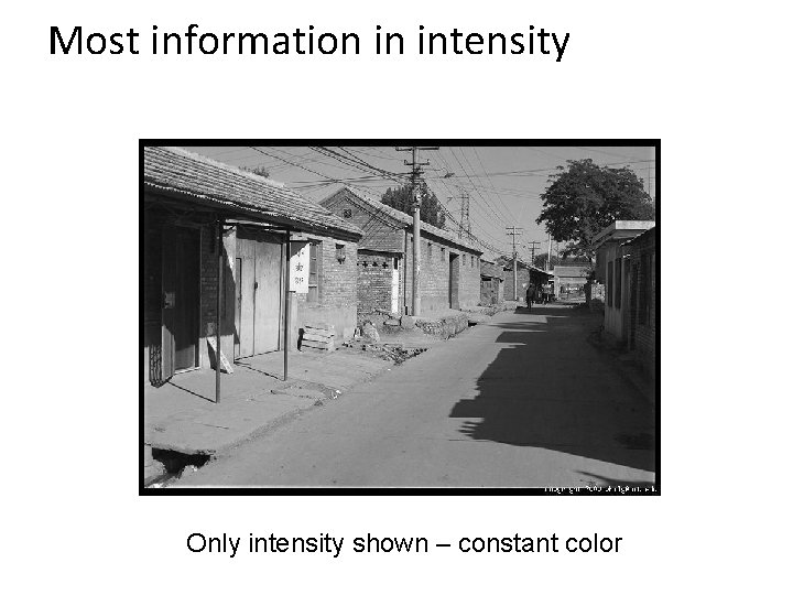
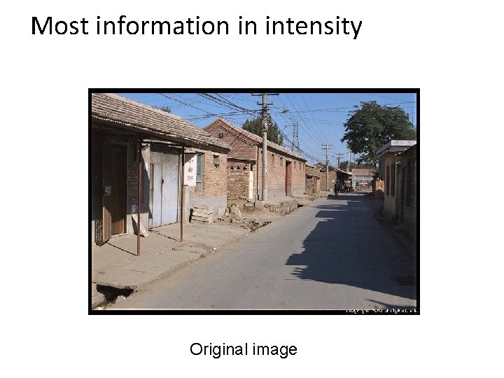
Which contains more information? (a) intensity (1 channel) (b) chrominance (2 channels)

Most information in intensity Only color shown – constant intensity

Most information in intensity Only intensity shown – constant color

Most information in intensity Original image

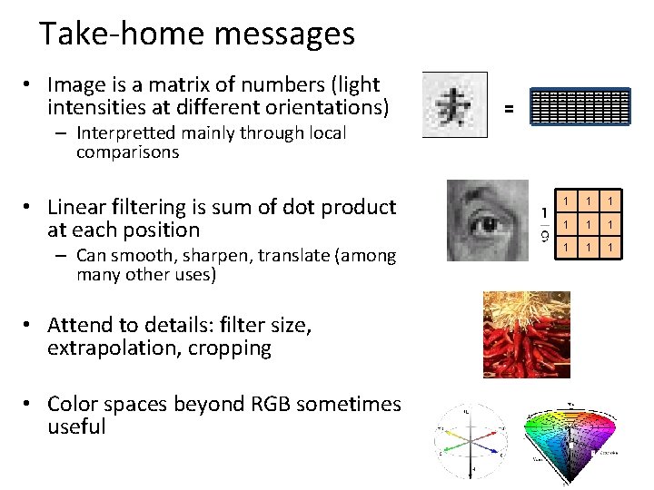
Take-home messages • Image is a matrix of numbers (light intensities at different orientations) – Interpretted mainly through local comparisons • Linear filtering is sum of dot product at each position – Can smooth, sharpen, translate (among many other uses) • Attend to details: filter size, extrapolation, cropping • Color spaces beyond RGB sometimes useful 0. 92 = 0. 93 0. 94 0. 97 0. 62 0. 37 0. 85 0. 97 0. 93 0. 92 0. 99 0. 95 0. 89 0. 82 0. 89 0. 56 0. 31 0. 75 0. 92 0. 81 0. 95 0. 91 0. 89 0. 72 0. 51 0. 55 0. 51 0. 42 0. 57 0. 41 0. 49 0. 91 0. 92 0. 96 0. 95 0. 88 0. 94 0. 56 0. 46 0. 91 0. 87 0. 90 0. 97 0. 95 0. 71 0. 81 0. 87 0. 57 0. 37 0. 80 0. 88 0. 89 0. 79 0. 85 0. 49 0. 62 0. 60 0. 58 0. 50 0. 61 0. 45 0. 33 0. 86 0. 84 0. 74 0. 58 0. 51 0. 39 0. 73 0. 92 0. 91 0. 49 0. 74 0. 96 0. 67 0. 54 0. 85 0. 48 0. 37 0. 88 0. 90 0. 94 0. 82 0. 93 0. 69 0. 49 0. 56 0. 66 0. 43 0. 42 0. 77 0. 73 0. 71 0. 90 0. 99 0. 73 0. 90 0. 67 0. 33 0. 61 0. 69 0. 73 0. 97 0. 91 0. 94 0. 89 0. 41 0. 78 0. 77 0. 89 0. 93 1 1 1 1 1